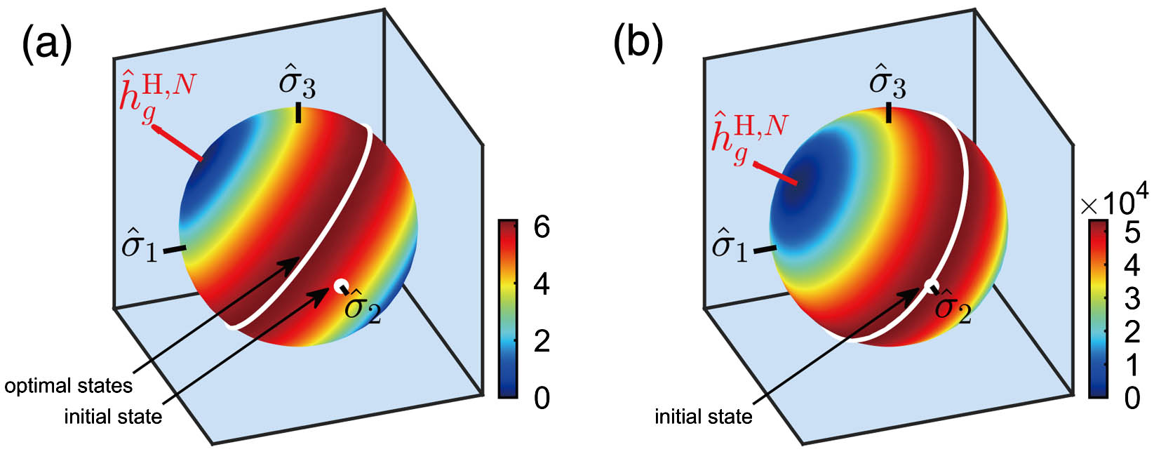
Fig. 1. Red vector represents the direction of the generated h^gH,N on the Bloch sphere. The white curve corresponds to the set of quantum states that are orthogonal to h^gH,N and maximize its variance. (a) At a small time scale of gt = 1, the eigenstates of σ^2 (marked as white dots) do not belong to the optimal state set. (b) At a longer time scale of gt = 100, the eigenstate of σ^2 lies on the white curve, indicating that the state is one of the optimal initial states. Here, we take N = 1 and Δ = 2g.

Fig. 2. Blue dashed line depicts the variation of FgO,bs with respect to the excitation number N. The blue solid line is for the limit case of small detuning, while the orange solid line represents the variation of variance ΔN² with respect to N. Here, we set N¯=10, gt = 100, and Δ = 100g.

Fig. 3. Density plot of R=FgP/FgO versus the phase difference and particle number fluctuation. (a) Large detuning with Δ = 200g. (b) Small detuning with Δ = 0 (resonance between the atom and the optical field). Other parameters are gt = 100 and n¯=100.

Fig. 4. FgP as a function of encoding time t for the different quantum states of optical fields, which (a) in the case of small detuning is Δ = 0 and (b) in the case of large detuning is Δ = 50g. The complex amplitude of the coherent state is α=20eiπ/2, and the corresponding atomic state is (|e〉+|g〉)/2. The squeezed amplitude of the squeezed states is r = 0.7. When the squeezed angles are θ = 0 (amplitude-squeezed state) and θ = π (phase-squeezed state), the corresponding atomic states are (|e〉+e−iπ/2|g〉)/2 and (|e〉+eiπ/2|g〉)/2, respectively. Importantly, for the sake of fairness, it is necessary to set the average number of photons to be the same for different optical field states, i.e., α=20−sinh(r)2.