• Chinese Optics Letters
  • Vol. 19, Issue 3, 031101 (2021)
Jie Dai1、2, Lihua Huang1、2、*, Kai Guo1, Liqing Ling1, and Huijie Huang1、2
Author Affiliations
  • 1Laboratory of Information Optics and Optoelectronic Technology, Shanghai Institute of Optics and Fine Mechanics, Chinese Academy of Sciences, Shanghai 201800, China
  • 2Center of Materials Science and Optoelectronics Engineering, University of Chinese Academy of Sciences, Beijing 100049, China
  • show less
    DOI: 10.3788/COL202119.031101 Cite this Article Set citation alerts
    Jie Dai, Lihua Huang, Kai Guo, Liqing Ling, Huijie Huang. Reflectance transformation imaging of 3D detection for subtle traces[J]. Chinese Optics Letters, 2021, 19(3): 031101 Copy Citation Text show less
    Image acquisition device and the distribution of the direction of the incident light.
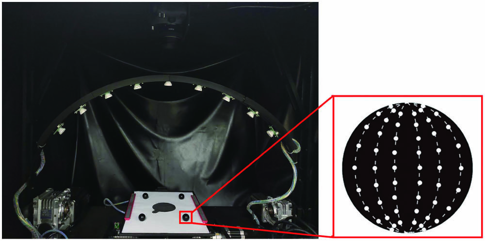
    Fig. 1. Image acquisition device and the distribution of the direction of the incident light.
    Sample and RTI reconstructions. (a) Original photo of the front. (b) RTI reconstruction of the front with specular enhancement. (c) Original photo of the back. (d) RTI reconstruction of the back with specular enhancement.
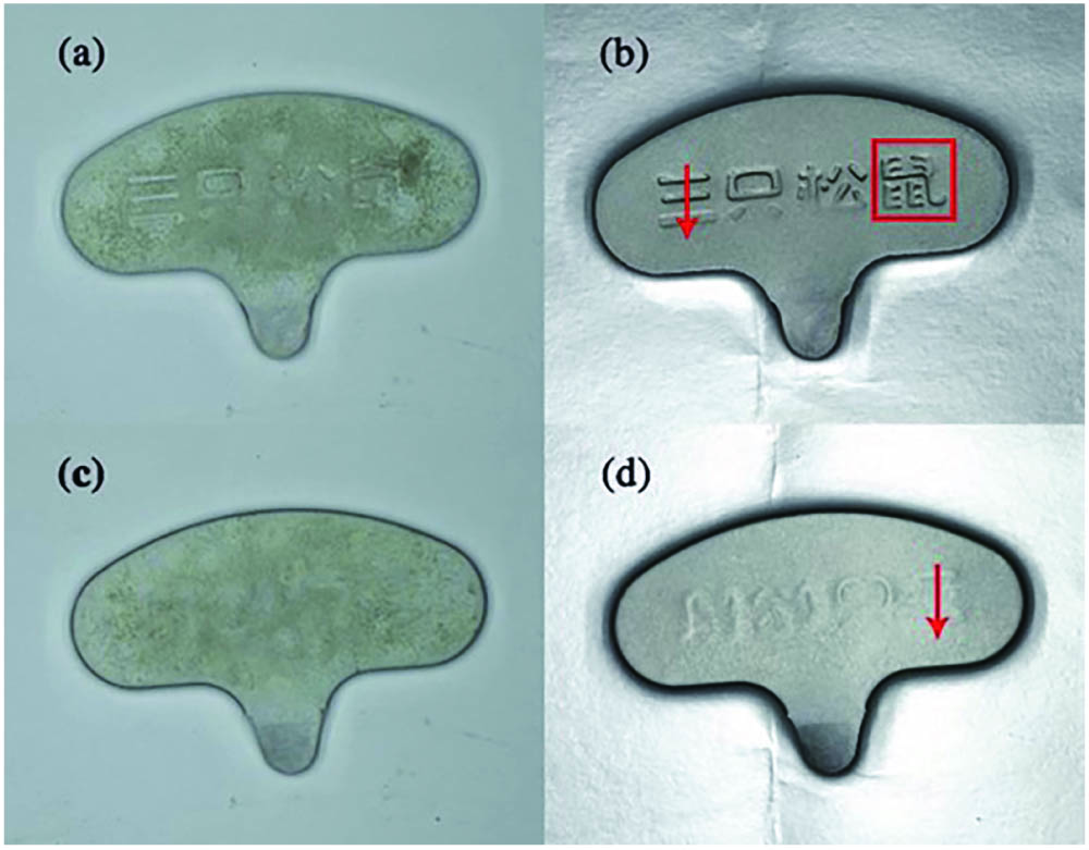
    Fig. 2. Sample and RTI reconstructions. (a) Original photo of the front. (b) RTI reconstruction of the front with specular enhancement. (c) Original photo of the back. (d) RTI reconstruction of the back with specular enhancement.
    Normal maps of the two sides of the metal in Fig. 2. (a) The normal map of the front. (b) The normal map of the back.
    Fig. 3. Normal maps of the two sides of the metal in Fig. 2. (a) The normal map of the front. (b) The normal map of the back.
    3D recovery results of the trace in the red box in Fig. 2(b). (a) Results without filtering normal data. (b) Recovery by PS algorithm after data filtering (T = 1, w = 0, k = 0, λ = 0). (c) Recovery using PS algorithm after data filtering and data conversion (T = 1, w = 0.5, k = 0, λ = 0). (d) The result of our algorithm (T = 1, w = 0.5, k = 0, λ = 1). (e) The planes taken from the same parts marked by different colors of the above reconstructions and MSEs of these parts. (f) The contours of the above reconstructions along the direction indicated by the colored arrows.
    Fig. 4. 3D recovery results of the trace in the red box in Fig. 2(b). (a) Results without filtering normal data. (b) Recovery by PS algorithm after data filtering (T = 1, w = 0, k = 0, λ = 0). (c) Recovery using PS algorithm after data filtering and data conversion (T = 1, w = 0.5, k = 0, λ = 0). (d) The result of our algorithm (T = 1, w = 0.5, k = 0, λ = 1). (e) The planes taken from the same parts marked by different colors of the above reconstructions and MSEs of these parts. (f) The contours of the above reconstructions along the direction indicated by the colored arrows.
    Different enhanced 3D topographies of the trace marked by red arrows in Fig. 2(d). (a) The 3D reconstruction without enhancement (k = 0). (b) The 3D topography enhanced by k = 15 and d = 15. (c) The 3D topography enhanced by k = 25 and d = 15. (d) The 3D topography enhanced by k = 25 and d = 25.
    Fig. 5. Different enhanced 3D topographies of the trace marked by red arrows in Fig. 2(d). (a) The 3D reconstruction without enhancement (k = 0). (b) The 3D topography enhanced by k = 15 and d = 15. (c) The 3D topography enhanced by k = 25 and d = 15. (d) The 3D topography enhanced by k = 25 and d = 25.
    (a) Metal back 3D reconstruction (w = 0.5, k = 25, d = 25, λ = 1). (b) Trace 3D reconstruction on the back (w = 0.5, k = 25, d = 25, λ = 1).
    Fig. 6. (a) Metal back 3D reconstruction (w = 0.5, k = 25, d = 25, λ = 1). (b) Trace 3D reconstruction on the back (w = 0.5, k = 25, d = 25, λ = 1).
    Scanning results with the DetakXT profilometer (128 µm scanning range, 1% accuracy) and depth recovery results of the same part. The scanning position and direction are shown as red arrows in Fig. 2. (a) Scanning results and depth recovery of Fig. 2(b), R2 = 0.8772. (b) Scanning results and depth recovery of Fig. 2(b), R2 = 0.9387.
    Fig. 7. Scanning results with the DetakXT profilometer (128 µm scanning range, 1% accuracy) and depth recovery results of the same part. The scanning position and direction are shown as red arrows in Fig. 2. (a) Scanning results and depth recovery of Fig. 2(b), R2 = 0.8772. (b) Scanning results and depth recovery of Fig. 2(b), R2 = 0.9387.
    Jie Dai, Lihua Huang, Kai Guo, Liqing Ling, Huijie Huang. Reflectance transformation imaging of 3D detection for subtle traces[J]. Chinese Optics Letters, 2021, 19(3): 031101
    Download Citation