
J. P. Trevino, V. Coello, A. Jaimes-Nájera, C. E. Garcia-Ortiz, S. Chávez-Cerda, J. E. Gómez-Correa, "Direct observation of longitudinal aberrated wavefields," Photonics Res. 11, 1015 (2023)
- Photonics Research
- Vol. 11, Issue 6, 1015 (2023)
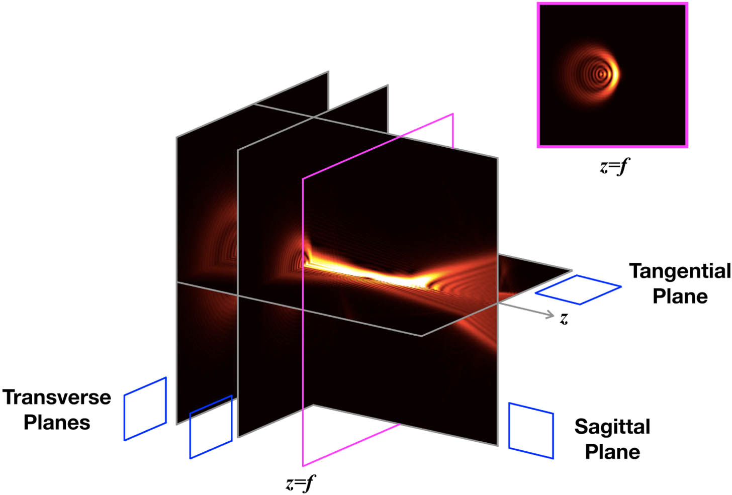
Fig. 1. 3D representation of a beam propagation. The beam is aberrated with coma; the main planes where the analyses take place are indicated with blue squares parallel to each plane.

Fig. 2. Each one of the Seidel terms for wave aberrations is plotted. The piston aberration is just a wave delay, while the tilt has a linear variation. The slope is proportional to the tilt angle of the incident beam. Defocus is a quadratic function and coma is cubic.
Fig. 3. How to adjust the system. The exit pupil plane is in yellow. The position of the sample relative to the Gaussian beam: (a) with the initial alignment to get an unaberrated field and with a displacement to get a defocused field and (b) with a tilt and a displacement to get tilted and comatic aberrations. This figure illustrates how there are regions of the wavefront arriving at the sample ahead of others, thus producing the desired Seidel aberrations. (c) Moving the beam is equivalent to moving the sample since the wavefront is incident on the plane with the same phase shifts.
Fig. 4. Image of an LRM system. The angle α α
Fig. 5. Aberration-free beam. (a) Incident Gaussian light beam focused with the 10 ×
Fig. 6. Tilting the incident beam. (a) Incident light beam focused with the 40 ×
Fig. 7. Defocused beam. (a) Incident light beam defocused with the 40 ×
Fig. 8. Coma-like beam. (a) Incident light beam defocused with the 40 ×


Set citation alerts for the article
Please enter your email address

© Copyright 2018-2021 | Chinese Laser Press. All Rights Reserved 沪ICP备15018463号-20