Derivative ghost imaging

Zhe Yang; Kexin Huang; Machi Zhang; Dong Ruan; Junlin Li

doi:10.3788/COL202220.011101

Abstract

We propose a new experimentally verified ghost imaging (GI) mechanism, derivative GI. Our innovation is that we use the derivatives of the intensities of the test light and the reference light for imaging. Experimental results show that by combining derivative GI with the standard GI algorithm, multiple independent signals can be obtained in one measurement. This combination greatly reduces the number of measurements and the time required for data acquisition and imaging. Derivative GI intrinsically does not produce the storage-consuming background term of GI, so it is suitable for on-chip implementation and makes practical application of GI easier.

Keywords

derivative ghost imaging derivative Hanbury Brown and Twiss effect derivative of intensity ghost imaging on-chip ghost imaging

1. Introduction

Ghost imaging (GI) is a non-local imaging technique that uses the second-order correlation function of light to obtain information about objects^[1–5]. GI requires two light paths for imaging: the test light interacts with the object and is received by the barrel detector; the reference light is received by the array detector. GI and the related fields of computational GI and single-pixel imaging have attracted widespread attention^[6–10]. Imaging in GI requires only a bucket detector for the test light beam. This gives GI an advantage over other techniques in areas in which array cameras are undesirable and in which nonvisible spectral bands are used, such as X-ray^[11], infrared^[12], and terahertz (THz)^[13]. GI is important in other applications^[14,15], such as lensless imaging^[16,17], 3D imaging^[18], lidar^[19], and encrypted communication^[20]. There have been many important developments that have improved image quality as the use of GI has increased; examples are differential GI (DGI)^[21], iterative GI^[22], and higher-order GI^[23]. The deterministic orthogonal basis scanning algorithms can perform high-quality imaging using the Hadamard basis or Fourier basis^[24–28]. Compressed sensing algorithms produce high-quality images at low sampling rates^[29,30]. The combination of GI and deep learning has recently been shown to improve image quality and reduce sampling times^[31–35].

Creating on-chip GI algorithms is a key step in the practical application of GI because it reduces the cost and allows high-volume use of GI. GI requires a large number of measurements, which creates three challenges for on-chip GI algorithms to overcome: (i) there are many measurements, so data acquisition is time-consuming; (ii) required memory storage is very large, which is difficult to ensure in on-chip implementation; (iii) the image reconstruction algorithm takes a long time to form the image of the object. In 2020, we proposed an instant GI (IGI) algorithm that overcame challenges (ii) and (iii). The use of IGI greatly reduces the storage space required for GI, and the imaging time is almost zero. This study represents for the first time, to the best of our knowledge, in the field of GI that GI has been implemented on a chip, freeing GI from some of the limitations imposed by the use of conventional computers^[36,37].

However, the IGI algorithm requires the same number of measurements as the standard GI algorithm to function at the same level. So, an algorithm is urgently needed that can both reduce the number of measurements and be suitable for on-chip implementation. In this study, we propose a new GI technique, derivative GI, to reduce the number of measurements and decrease the time taken for data acquisition. We make innovative use of the derivatives of the intensities of the test light and the reference light for imaging, and we have experimentally verified the effectiveness of this novel technique.

Sign up for Chinese Optics Letters TOC. Get the latest issue of Chinese Optics Letters delivered right to you！Sign up now

Our experimental results show that by combining derivative GI with the standard GI algorithm, multiple independent signals can be obtained in a single measurement. This approach greatly reduces the number of measurements required for imaging and improves image quality. Furthermore, derivative GI intrinsically does not have the storage-consuming background term of GI. Therefore, the derivative GI is suitable to apply to on-chip GI. Derivative GI overcomes a significant obstacle in the engineering application of GI and is therefore of major importance in the practical application of GI.

2. Methods

2.1. Theory

In essence, GI depends on the Hanbury Brown–Twiss (HBT) effect for any two spatial points. We propose and experimentally demonstrate derivative HBT. We show that combining derivative HBT with standard HBT can reduce the number of measurements required for correlation.

Derivative HBT is described by $G_{HBT_Der}^{(2)} (x_{1}, x_{2}) = 〈 I^{(n)} (x_{1}) I^{(n)} (x_{2}) 〉,$ (1)where $x_{1}$ and $x_{2}$ are the spatial coordinates of different detectors, $I^{(n)} (x_{1})$ and $I^{(n)} (x_{2})$ are respectively the $n$ th-order derivatives of the measured intensities at $x_{1}$ and $x_{2}$ .

In particular, when $n = 1$ , the equation for the first-order derivative HBT can be obtained from Eq. (2): $G_{HBT_Der}^{(2)} (x_{1}, x_{2}) = 〈 I^{'} (x_{1}) I^{'} (x_{2}) 〉,$ (2)where $I^{'} (x_{1})$ and $I^{'} (x_{2})$ are, respectively, the first-order derivatives of the measured intensities at $x_{1}$ and $x_{2}$ .

It should be emphasized that all derivatives in this paper are derivates with respect to time $t$ . Therefore, $(n)$ represents $d^{(n)} / d t^{(n)}$ , and $'$ represents $d / d t$ .

For GI, derivative GI is given by $G_{Der}^{(2)} (x) = 〈 S^{(n)} I^{(n)} (x) 〉,$ (3)where $S^{(n)}$ is the $n$ th derivative of the intensity of the bucket detector, and $I^{(n)} (x)$ is the $n$ th derivative of the intensity of the reference detector with the spatial coordinate $x$ .

In particular, when $n = 1$ , the equation for the first-order derivative GI can be obtained from Eq. (3): $G_{Der}^{(2)} (x) = 〈 S^{'} I^{'} (x) 〉,$ (4)where $S^{'}$ is the first derivative of the intensity at the bucket detector, and $I^{'} (x)$ is the first derivative of the intensity of the reference light at the spatial coordinate $x$ .

2.2. Experimental setup

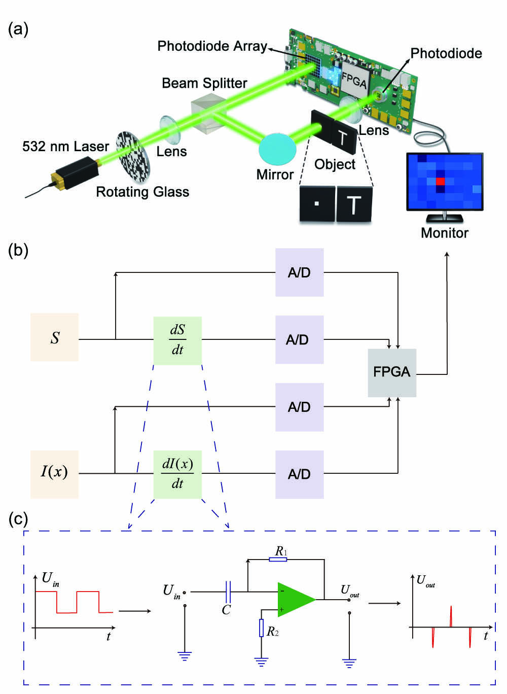
The experimental configuration is shown in Fig. 1. The 532 nm laser is projected onto the light-modulation glass disk to produce pseudo-thermal light. The pseudo-thermal light is split into two beams by the beam splitter. The test beam is directed onto the object, and light that passes through the object is received by the bucket detector; the reference beam is received directly by the array detector. The detector was a Hamamatsu S13620 array detector with $8 \times 8$ pixels capable of high-speed sampling of the derivative signal. A lens and one pixel in another S13620 array were used as the bucket detector. The switching speed of the pattern and the sampling frequency of the analog-to-digital converter (A/D) were both about 100 kHz.

Figure 1.Experimental schematic. (a) The pseudo-thermal light is generated by a 532 nm laser illuminating a rotating light-modulating glass disk. The HBT experiment used a small hole in the object plane, and the GI experiment used the letter T as the object. (b) The bucket detector signal S and the reference light signal I(x) are received by the photodetectors to produce a photocurrent. The photocurrent is sampled by the analog-to-digital converter (A/D) to obtain S and I(x), and is transmitted to the field programmable gate array (FPGA). Simultaneously, the photocurrents enter the differentiators to produce the derivative signals, which then undergo A/D sampling and are transmitted to the FPGA for calculation of the experimental results. In the HBT experiment, the signal flow is similar to (b), with I(x₁) and I(x₂) replacing S and I(x). (c) The differentiators for S and I(x) are implemented by differentiating the operational amplitude circuits.

The distance from the glass to the object was equal to the distance from the glass to the detector array. The HBT effect was obtained using a small square hole in the object plane that allowed only light collected by one pixel to pass. The GI experiment used the letter T in the object plane.

We developed a configurable hardware system that sampled both the intensity and its first-order derivative [shown as the circuit board in Fig. 1(a)]. In the standard GI experiment, the signal was immediately sampled by the A/D and then transmitted to the field programmable gate array (FPGA). In the derivative GI experiment, the signal was initially sent to the differentiator to produce the derivative signal, which was then sampled by the A/D and transmitted to the FPGA for calculation of the correlations, as shown in Fig. 1(b). The HBT experiment used an identical configuration, but $I (x_{1})$ and $I (x_{2})$ were replaced by $S$ and $I (x)$ .

All measured data of the derivative HBT and derivative GI were processed online immediately by the FPGA. When measurement ended, the correlation results were immediately available.

3. Experimental Results

Figure 2(a) shows the result of the first-order derivative HBT experiment, and Fig. 2(b) shows the result of the standard HBT experiment. The number of measurements was $M = 512$ for each experiment. It can be seen that the first-order derivative HBT and the standard HBT have very similar correlation characteristics. In order to compare the derivative HBT and standard HBT easily, we subtracted the background term ( $〈 I (x_{1}) 〉 〈 I (x_{2}) 〉$ ) of the standard HBT and rescaled the values of the two sets of experimental results to the same level. In this paper, we use $G_{rescale} (x) = G (x) / | \min (G) |$ to rescale the results of standard GI (HBT) and derivative GI (HBT) to the same level.

Figure 2.Experimental results of (a) the first-order derivative HBT and (b) standard HBT. The number of measurements M in both cases was 512.

Figure 3(a) shows the object letter T; transmission through the white part was recorded as 1, and transmission through the black part was recorded as 0. The pixel size of the transparent part of the object was $3 mm \times 3 mm$ , and the pixel array was $8 \times 8$ . Figure 3(b) shows the image of the object obtained by the first-order derivative GI ( $M = 1024$ ), and Fig. 3(c) shows the image of the object obtained by standard GI ( $M = 1024$ ). It can be seen that the image quality of the first-order derivative GI is very similar to that of the standard GI.

Figure 3.(a) Object of the GI experiment, and the experimental results of (b) the first-order derivative GI and (c) standard GI. The number of measurements M in each case was 1024.

The signal-to-noise ratio (SNR) is $SNR = \frac{〈 I_{S} 〉 - 〈 I_{N} 〉}{(σ_{s} + σ_{N}) / 2},$ (5)where $〈 I_{S} 〉$ and $〈 I_{N} 〉$ are the average values of intensities of the object region (letter ‘T’) and the background region [blue dash ‘T’ in Fig. 3(a)] in the image; $σ_{S}$ and $σ_{N}$ are the standard derivations of intensities of the object region and the background region and are widely used to measure the image quality of GI^[38]. The average SNR is obtained by 10 times experiments.

We want to emphasize that the derivative GI does not produce the background term ( $〈 S 〉 〈 I (x) 〉$ ), which is storage-consuming, because the derivative of the intensity signal intrinsically removes the direct current (DC) photocurrent component, which requires large memory space. This is the reason why derivative GI is suitable for on-chip implementation and does not need a computer.

In order to compare the derivative GI and standard GI easily, we subtracted the background term ( $〈 S 〉 〈 I (x) 〉$ ) of the standard GI and rescaled the values of the two sets of experimental results to the same level.

We now demonstrate that the first-order derivative HBT can be combined with standard HBT to reduce the number of experimental samples taken and show that data with different degrees of freedom can be obtained from one measurement. Figure 4(a) shows the first-order derivative HBT result ( $M = 256$ ), and Fig. 4(b) shows the result of standard HBT ( $M = 256$ ). Figure 4(c) shows the combination of data in Figs. 4(a) and 4(b); data were rescaled and then summed. It can be seen that the combination of first-order derivative HBT and standard HBT significantly improved the strength of the correlation. Although the number of measurements was only 256, it is obvious by comparing Figs. 4(c) and 2(b) that the correlation of intensity after combination was very similar to the correlation obtained by 512 measurements of the standard HBT effect.

Figure 4.Experimental results of (a) the first-order derivative HBT, (b) standard HBT (the number of measurements M in each case was 256), and (c) combination of (a) and (b) by simple addition after rescaling. The experimental results of (d) first-order derivative GI, (e) standard GI (the number of measurements M in each case was 512), and (f) the combination of (d) and (e).

Similarly, Figs. 4(d)–4(f) show that derivative GI [Fig. 4(d)] can be combined with standard GI [Fig. 4(f)] to reduce the number of image sample measurements and significantly improve image quality. A comparison of Figs. 4(f) and 3(c) shows that the combined image quality, from 512 measurements, is as good as the image quality of the standard GI algorithm from 1024 measurements.

The combination result is obtained by $G_{combine} = [G_{GI} / | \min (G_{GI}) |] / 2 + [G_{Der_GI} / | \min (G_{Der_GI}) |] / 2 .$ (6)

Figure 5 shows the SNR results of the standard GI, the first-order derivative GI, and the combination of the two with different numbers of measurements. Each point with an error bar is calculated by 10 repeated experimental results. It can be seen from Fig. 5 that the image quality of standard GI and derivative GI is at the same level. For the same measurement number, the SNR of the combination is obviously better than that of any GI alone. Moreover, with increasing $M$ , the SNR results of three algorithms increase.

Figure 5.Experimental results of the standard GI, the first-order derivative GI, and the combination of the two within different sample numbers M.

To validate the independence of the light intensity with its derivative signal, the experimental results of the correlation $〈 I (x_{0}) I^{'} (x) 〉 - 〈 I (x_{0}) 〉 〈 I^{'} (x) 〉$ are shown in Fig. 6. Different $x_{0}$ have been checked, although two of them are displayed. It can be seen that the random intensity and its derivative signal have no correlation. If $〈 I (x_{0}) 〉$ and $〈 I^{'} (x_{0}) 〉$ , which are obtained from the same measurements, have correlations, it should get results similar to the HBT effect. However, no obvious correlation signal is obtained.

Figure 6.Experimental results of 〈I (x₀)I′(x)〉 − 〈I (x₀)〉〈I′ (x)〉. x₀ is chosen as (a) row 3 and column 3 and (b) row 5 and column 5, respectively.

4. Discussion

Because the signal strength $S$ ( $I (x)$ ) and its derivative $S^{'}$ ( $I^{'} (x)$ ) differ in degrees of freedom, the combination of derivative GI and standard GI reduces the number of measurements and increases the associated signal strength, while standard GI alone only measures the degree of freedom of intensity at one time. Our solution, in combining the two effects, adds the degree of freedom of the derivative, which indicates that one measurement provides two independent data items. Furthermore, if we could detect the intensity, the first derivative, the second derivative, and on to the $N$ th-order derivative at the same time, it would mean that a single measurement could provide $N + 1$ independent sets of information. This would greatly improve the efficiency of experiments and reduce the data-acquisition time, which is very important for practical application of GI.

GI can be regarded as the achievement of $O (x) = 〈 δ S δ I (x) 〉 = 〈 (S - 〈 S 〉) (I (x) - 〈 I (x) 〉) 〉$ . For the standard GI, the $S$ and $I (x)$ are measured. Afterwards, $〈 S I (x) 〉$ subtracts $〈 S 〉 〈 I (x) 〉$ to achieve $〈 δ S δ I (x) 〉$ to obtain the image of the object. For the derivative GI with $〈 S^{'} 〉 = 0$ and $〈 I^{'} (x) 〉 = 0$ , the $S^{'}$ and $I^{'} (x)$ are obtained by the hardware system. It can be seen that the $〈 S^{'} I^{'} (x) 〉$ is intrinsically $〈 δ S δ I (x) 〉$ . In other words, the $〈 δ S δ I (x) 〉$ is directly achieved by $〈 S^{'} I^{'} (x) 〉$ without calculating $〈 S^{'} 〉 〈 I^{'} (x) 〉$ .

$I^{'} (x)$ can be seen as a random variable with $〈 I^{'} (x) 〉 = 0$ , and $I (x)$ can be taken as a random variable with a background/DC term, where $〈 I (x) 〉 \neq 0$ . Because the $I (x)$ and its derivative $I^{'} (x)$ are independent random variables, the combination of standard GI and the first-order derivative GI with the number of measurements $M$ can be seen as $2 M$ measurements. Theoretically, image quality of GI with $2 M$ measurements is better than that with $M$ measurements. Therefore, the combination of the two can improve the image quality of GI.

Some algorithms such as DGI, normalized GI, and higher-order GI can also improve the image quality of GI. There are two reasons why the derivative GI is more suitable for the on-chip implementation of GI. First, the derivative GI does not require one matrix to store the $〈 I (x) 〉$ to calculate $〈 S 〉 〈 I (x) 〉$ . Second, the speed of the numerical accumulation of the $〈 S^{'} I^{'} (x) 〉$ is much less than that of $〈 S I (x) 〉$ ^[36]. This is particularly important in the implementation of on-chip GI, because the value of the element of the storage matrix cannot be very large for on-chip GI with extremely limited hardware resources^[37]. Furthermore, DGI mainly works in the cases of the ratio between the obstacle area and the beam size being small^[21]. Derivative GI does not have this limit.

In 1956, Hanbury Brown and Twiss used the second-order correlation of light intensity to measure the angular diameter of Sirius. The second-order correlation of intensity is known as the HBT effect^[39,40], and it has important applications in the fields of astronomy^[41,42], nuclear physics^[43,44], condensed matter^[45,46], and quantum optics^[47–50]. Since the HBT effect was discovered in 1956, it has been used mainly in the correlation of intensity. We innovated by expanding the theory underlying the HBT effect, and we proposed a new formulation of HBT, derivative HBT, which uses the correlation of derivatives of intensity to produce a correlation effect similar to the standard HBT effect. We experimentally demonstrated derivative HBT and showed that combining derivative HBT with standard HBT can reduce the number of measurements required for correlation when using only HBT. This reduction greatly increased experimental efficiency, reduced experimental difficulty, and made possible experiments that were previously infeasible. Derivative HBT has important applications in the fields of astronomy, nuclear physics, condensed matter, and quantum optics.

5. Conclusions

In summary, we proposed the innovative derivative GI model and obtained image quality the same as standard GI. The importance of derivative GI is seen when the correlation results are combined with those of standard GI; signals with multiple degrees of freedom can be obtained in one measurement. Combining the intensity with its derivative reduces the number of measurements required and thus data-acquisition time. Moreover, derivative GI can be applied to on-chip GI because it intrinsically does not produce the storage-consuming background term of GI and is suitable for on-chip implementation.

We used experiments to show the effectiveness of first-order derivative GI and first-order derivative HBT. The method of using first-order derivative GI and higher-order derivative GI that we demonstrated will promote greater practical application of GI in many areas.

References

[1] T. B. Pittman, Y. H. Shih, D. V. Strekalov, A. V. Sergienko. Optical imaging by means of two-photon quantum entanglement. Phys. Rev. A, 52, R3429(1995).

[2] R. S. Bennink, S. J. Bentley, R. W. Boyd. ‘Two-photon’ coincidence imaging with a classical source. Phys. Rev. Lett., 89, 113601(2002).

[3] A. Gatti, E. Brambilla, M. Bache, L. A. Lugiato. Ghost imaging with thermal light: comparing entanglement and classical correlation. Phys. Rev. Lett., 93, 093602(2004).

[4] F. Ferri, D. Magatti, A. Gatti, M. Bache, E. A. Brambilla, L. A. Lugiato. High-resolution ghost image and ghost diffraction experiments with thermal light. Phys. Rev. Lett., 94, 183602(2005).

[5] D. Z. Cao, J. Xiong, K. Wang. Geometrical optics in correlated imaging systems. Phys. Rev. A, 71, 013801(2005).

[6] J. H. Shapiro. Computational ghost imaging. Phys. Rev. A, 78, 061802(2008).

[7] O. Katz, B. Yaron, Y. Silberberg. Compressive ghost imaging. Appl. Phys. Lett., 95, 131110(2009).

[8] G. M. Gibson, S. D. Johnson, M. Padgett. Single-pixel imaging 12 years on: a review. Opt. Express, 28, 28190(2020).

[9] Z. Yang, O. S. Magana-Loaiza, M. Mirhosseini, Y. Zhou, B. Gao, L. Gao, S. M. H. Rafsanjani, G. L. Long, R. W. Boyd. Digital spiral object identification using random light. Light: Sci. Appl., 6, e17013(2017).

[10] L. Wang, S. Zhao. Super resolution ghost imaging based on Fourier spectrum acquisition. Opt. Laser. Eng., 139, 106473(2021).

[11] X. Zhang, Y. H. He, L. A. Wu, L. M. Chen, B. B. Wang. Tabletop x-ray ghost imaging with ultra-low radiation. Optica, 5, 374(2018).

[12] N. Radwell, K. J. Mitchell, G. M. Gibson, M. P. Edgar, R. Bowman, M. J. Padgett. Single-pixel infrared and visible microscope. Optica, 1, 285(2014).

[13] J. Zhao, E. Yiwen, K. Williams, X. C. Zhang, R. Boyd. Spatial sampling of terahertz fields with sub-wavelength accuracy via probe beam encoding. Light: Sci. Appl., 8, 55(2019).

[14] G. Wang, H. Zheng, Z. Tang, Y. He, Y. Zhou, H. Chen, J. Liu, Y. Yuan, F. Li, Z. Xu. Naked-eye ghost imaging via photoelectric feedback. Chin. Opt. Lett., 18, 091101(2020).

[15] J. Gu, S. Sun, Y. Xu, H. Lin, W. Liu. Feedback ghost imaging by gradually distinguishing and concentrating onto the edge area. Chin. Opt. Lett., 19, 041102(2021).

[16] L. Basano, P. Ottonello. Experiment in lensless ghost imaging with thermal light. Appl. Phys. Lett., 89, 091109(2006).

[17] Z. Yang, L. Zhao, X. Zhao, W. Qin, J. Li. Lensless ghost imaging through the strongly scattering medium. Chin. Phys. B, 25, 024202(2016).

[18] M. J. Sun, M. P. Edgar, G. M. Gibson, B. Sun, N. Radwell, R. Lamb, M. J. Padgett. Single-pixel three-dimensional imaging with time-based depth resolution. Nat. Commun., 7, 12010(2016).

[19] W. Gong, C. Zhao, H. Yu, M. Chen, W. Xu, S. Han. Three-dimensional ghost imaging lidar via sparsity constraint. Sci. Rep., 6, 26133(2016).

[20] Y. Wang, H. Chen, W. Jiang, X. Li, X. Chen, X. Meng, P. Tian, B. Sun. Optical encryption for visible light communication based on temporal ghost imaging with a micro-LED. Opt. Laser. Eng., 134, 106290(2020).

[21] F. Ferri, D. Magatti, L. A. Lugiato, A. Gatti. Differential ghost imaging. Phys. Rev. Lett., 104, 253603(2010).

[22] X. R. Yao, W. K. Yu, X. F. Liu, L. Z. Li, M. F. Li, L. A. Wu, G. J. Zhai. Iterative denoising of ghost imaging. Opt. Express, 22, 24268(2014).

[23] S. S. Hodgman, W. Bu, S. B. Mann, R. I. Khakimov, A. G. Truscott. Higher-order quantum ghost imaging with ultracold atoms. Phys. Rev. Lett., 122, 233601(2019).

[24] C. M. Watts, D. Shrekenhamer, J. Montoya, G. Lipworth, J. Hunt, T. Sleasman, S. Krishna, D. R. Smith, W. J. Padilla. Terahertz compressive imaging with metamaterial spatial light modulators. Nat. Photon., 8, 605(2014).

[25] Z. Zhang, X. Ma, J. Zhong. Single-pixel imaging by means of Fourier spectrum acquisition. Nat. Commun., 6, 6225(2015).

[26] K. M. Czajkowski, A. Pastuszczak, R. Kotynski. Real-time single-pixel video imaging with Fourier domain regularization. Opt. Express, 26, 20009(2018).

[27] L. Wang, S. Zhao. Fast reconstructed and high-quality ghost imaging with fast Walsh–Hadamard transform. Photon. Res., 4, 240(2016).

[28] Z. H. Xu, W. Chen, J. Penuelas, M. J. Padgett, M. J. Sun. 1000 fps computational ghost imaging using LED-based structured illumination. Opt. Express, 26, 2427(2018).

[29] J. Liu, J. Zhu, C. Lu, S. Huang. High-quality quantum-imaging algorithm and experiment based on compressive sensing. Opt. Lett., 35, 1206(2010).

[30] J. Liu. On the recovery conditions for practical ghost imaging with AMP algorithm. Opt. Express, 26, 20519(2018).

[31] H. Wu, R. Wang, G. Zhao, H. Xiao, X. Zhang. Sub-Nyquist computational ghost imaging with deep learning. Opt. Express, 28, 3846(2020).

[32] F. Wang, H. Wang, H. Wang, G. Li, G. Situ. Learning from simulation: an end-to-end deep-learning approach for computational ghost imaging. Opt. Express, 27, 25560(2019).

[33] H. Wu, G. Zhao, M. Chen, L. Cheng, H. Xiao, L. Xu, D. Wang, J. Liang, Y. Xu. Hybrid neural network-based adaptive computational ghost imaging. Opt. Laser. Eng., 140, 106529(2021).

[34] H. Wu, R. Wang, G. Zhao, H. Xiao, J. Liang, D. Wang, X. Tian, L. Cheng, X. Zhang. Deep-learning denoising computational ghost imaging. Opt. Laser. Eng., 134, 106183(2020).

[35] T. Bian, Y. Yi, J. Hu, Y. Zhang, Y. Wang, L. Gao. A residual-based deep learning approach for ghost imaging. Sci. Rep., 10, 1(2020).

[36] Z. Yang, W. X. Zhang, Y. P. Liu, D. Ruan, J. L. Li. Instant ghost imaging: algorithm and on-chip implementation. Opt. Express, 28, 3607(2020).

[37] Z. Yang, W. X. Zhang, M. C. Zhang, D. Ruan, J. L. Li. Instant ghost imaging: improving robustness for ghost imaging on optical background noise. OSA Continuum, 3, 391(2020).

[38] M. J. Sun, H. Y. Wang, J. Y. Huang. Improving the performance of computational ghost imaging by using a quadrant detector and digital micro-scanning. Sci. Rep., 9, 4105(2019).

[39] R. H. Brown, R. Q. Twiss. Correlation between photons in two coherent beams of light. Nature, 177, 27(1956).

[40] R. H. Brown, R. Q. Twiss. A test of a new type of stellar interferometer on sirius. Nature, 178, 1046(1956).

[41] R. H. Miller. Measurement of stellar diameters. Science, 153, 581(1966).

[42] G. Baym. The physics of Hanbury Brown–Twiss intensity interferometry: from stars to nuclear collisions. Acta Phys. Pol. B, 29, 1839(1998).

[43] E. Frodermann, U. Heinz. Photon Hanbury Brown–Twiss interferometry for noncentral heavy-ion collisions. Phys. Rev. C, 80, 044903(2009).

[44] C. Plumberg, U. Heinz. Probing the properties of event-by-event distributions in Hanbury Brown–Twiss radii. Phys. Rev. C, 92, 044906(2015).

[45] M. Schellekens, R. Hoppeler, A. Perrin, J. V. Gomes, D. Boiron, A. Aspect, C. I. Westbrook. Hanbury Brown Twiss effect for ultracold quantum gases. Science, 310, 648(2005).

[46] H. Cayla, S. Butera, C. Carcy, A. Tenart, G. Hercé, M. Mancini, A. Aspect, I. Carusotto, D. Clément. Hanbury Brown and Twiss bunching of phonons and of the quantum depletion in an interacting Bose gas. Phys. Rev. Lett., 125, 165301(2020).

[47] Y. Bromberg, Y. Lahini, E. Small, Y. Silberberg. Hanbury Brown and Twiss interferometry with interacting photons. Nat. Photon., 4, 721(2010).

[48] J. Leach, B. Jack, J. Romero, A. K. Jha, A. M. Yao, S. Franke-Arnold, D. G. Ireland, R. W. Boyd, S. M. Barnett, M. J. Padgett. Quantum correlations in optical angle–orbital angular momentum variables. Science, 329, 662(2010).

[49] S. Hong, R. Riedinger, I. Marinković, A. Wallucks, S. G. Hofer, R. A. Norte, M. Aspelmeyer, S. Gröblacher. Hanbury Brown and Twiss interferometry of single phonons from an optomechanical resonator. Science, 358, 203(2017).

[50] T. Thomay, S. V. Polyakov, O. Gazzano, E. Goldschmidt, Z. D. Eldredge, T. Huber, V. Loo, G. S. Solomon. Simultaneous, full characterization of a single-photon state. Phys. Rev. X, 7, 041036(2017).