
Zhi-Jian LI, Feng-Bao YANG, Yu-Bin GAO, Lin-Na JI, Peng HU. Fusion method for infrared and other-type images based on the multi-scale Gaussian filtering and morphological transform[J]. Journal of Infrared and Millimeter Waves, 2020, 39(6): 810
- Journal of Infrared and Millimeter Waves
- Vol. 39, Issue 6, 810 (2020)
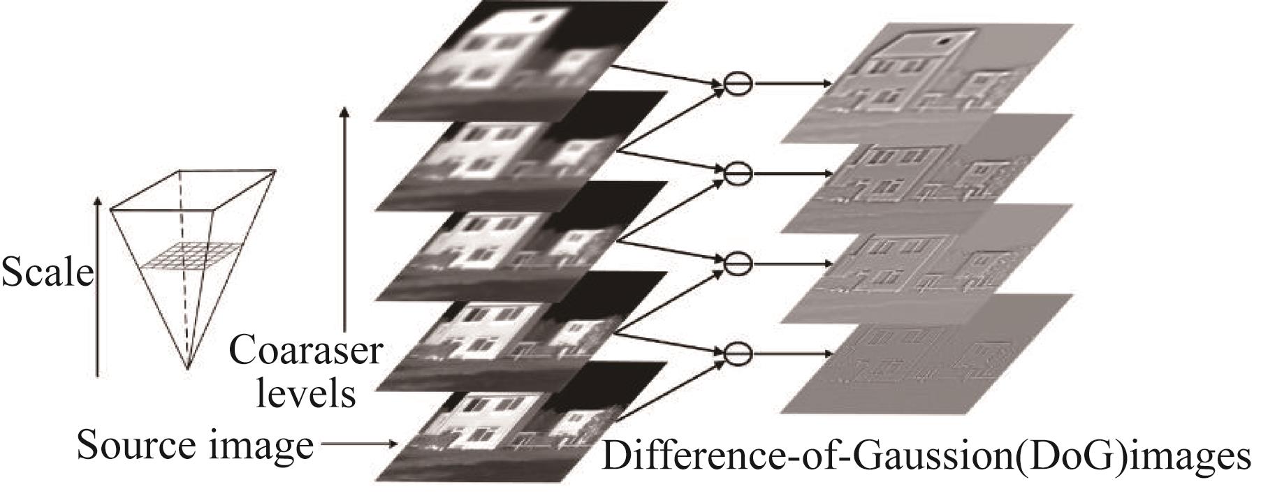
Fig. 1. Example of four-level decomposition by multi-scale Gaussian filtering
![[in Chinese]](/richHtml/hwyhmb/2020/39/6/810/img_2.png)
Fig. 2. [in Chinese]
Fig. 3. [in Chinese]
Fig. 4. The two kinds of source images (a) infrared-visible images, (b) infrared intensity-polarization images
Fig. 5. [in Chinese]
Fig. 6. Fusion results of one pair of the infrared-visible images (a) infrared image, (b) visible image, (c)-(i) the fusion results of the DWT, DTCWT, SWT, WPT, NSCT, NSST, and the proposed methods.
Fig. 7. Fusion results of one pair of the infrared intensity-polarization images (a) Infrared intensity image, (b) Infrared polarization image, (c)-(i) the fusion results of the DWT, DTCWT, SWT, WPT, NSCT, NSST, and the proposed methods.
|
Table 1. The parameters set in the compared methods. ‘Filter’ represents the Orientation filter; ‘Levels’ denotes the decomposition levels and the corresponding number of orientations for each level.
| |||||||||||||||
Table 2. The parameters of the proposed method for the four kinds of source images.
|
Table 3. Objective assessment of all methods (the best result of each metric is highlighted in bold).
|
Table 4. Average processing time (unit: sec.) comparison of eight methods. Each value represents the average run time of a frame in a certain sequence.

Set citation alerts for the article
Please enter your email address
© Copyright 2018-2021 | Chinese Laser Press. All Rights Reserved 沪ICP备15018463号-20