
Zhi-Jian LI, Feng-Bao YANG, Yu-Bin GAO, Lin-Na JI, Peng HU. Fusion method for infrared and other-type images based on the multi-scale Gaussian filtering and morphological transform[J]. Journal of Infrared and Millimeter Waves, 2020, 39(6): 810
- Journal of Infrared and Millimeter Waves
- Vol. 39, Issue 6, 810 (2020)
Abstract
Introduction
Visible, infrared, and infrared polarization images individually captured by different sensors present complementary information of the same scene, and they could be combined by the image fusion technology to obtain a new, more accurate, comprehensive, and reliable image description of the scene [
For the decomposition schemes, various methods are proposed, like the discrete wavelet transform (DWT) [
Fusion rules generally include low and high frequency coefficients fusion rules. The AVG-ABS rule is a simple fusion rule which uses the average rule to combine low-frequency coefficients and uses the absolute maximum rule to combine the high-frequency coefficients. The AVG-ABS fusion rule is computed easily and implemented simply, however, it always causes distortions and artifacts [
To ensure both the fusion quality and computational efficiency simultaneously, a novel multi-scale decomposition-based fusion method with dual decomposition structures is proposed. Our method is dedicated to improving the image fusion quality and efficiency from the aspect of image decomposition scheme, while for the rule aspect, our method only uses simple AVG-ABS rule. Firstly, inspired by the idea of constructing octaves in SIFT [
1 Related theories and work
1.1 The pyramid transforms
The theory and mathematical representation for constructing multiresolution pyramid transform scheme are presented by Ref.25 and extended by Ref.26. A domain of signals is assigned at each level, the analysis operators maps an image to a higher level in the pyramid, while the synthesis operator maps an image to a lower level in the pyramid, i.e. and . The detail signal contains information of x which does not exist in , where and is a subtraction operator mapping into the set . The decomposition process of an input image f is expressed as Eq.1:
where
And the reconstruction process through the backward recursion is expressed as Eq.3:
Eq.1 and Eq.3 are called the pyramid transform and the inverse pyramid transform respectively.
1.2 Scale space representation and multi-scale Gaussian filtering
The scale space of an image can be generated through convolving the image with Gaussian filters, and it has been successfully applied in SIFT [
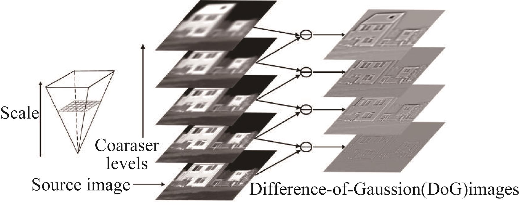
Inspired by the above algorithms, we have the source image repeatedly convolved with Gaussian filters whose standard deviation and size increase simultaneously to construct undecimated pyramid structure. Then, the DoG images are produced by subtracting adjacent Gaussian images. Accordingly, the transform scheme of such pyramid is given by Eq.4:
where
is the Gaussian kernels (filters) with a size of in this paper, and denotes the convolution operation. The parameter is the standard deviation, which is increasing with , and in this paper . Then the source image f can be decomposed into an approximation image and a set of detail images as shown in scheme 1, and it can also be exactly reconstructed through the following recursion:
The four-level decomposition scheme is illustrated in Fig.1.
![]()
Figure 1.Example of four-level decomposition by multi-scale Gaussian filtering
1.3 Multi-scale morphological transforms
The multi-scale top-hat transform using structuring elements with up-scaling size can extract the light and dark details at different image scales in image fusion [
The multi-scale morphological bottom-hat transform and its inverse are shown as follows
where the analysis operator is morphological closing operation , with also increasing with . The morphological outer-boundary transform and its inverse are similar to the bottom-hat transform and its inverse, with being replaced by dilation operation .
2 Proposed method framework
The proposed fusion method comprises three processes that are multi-scale decomposition, fusion, and reconstruction.
2.1 Multi-scale decomposition process
The K-level decomposition of a given source image by the scheme (4) has the form
where represents the detail image at level and denotes the approximation image of this multi-scale structure.
is a coarse representation of and usually inherit a few bright and dark details, thus the multi-scale top- and bottom-hat decompositions are used to extract bright objects on a dark background and dark objects on a bright background of different scales, respectively. Henceforth, can be decomposed by schemes mentioned in subsection 1.3 as
where and represent the detail images at level l obtained by the top- and bottom-hat decomposition process, respectively. And and denote the approximation images of the multi-scale top- and bottom-hat structure, respectively. Figure 2 is given as an example of three-level top- and bottom-hat decompositions.
![]()
Figure 2.
The detail image in scheme 9 comprises various details like edges and lines, thus the multi-scale inner- and outer-boundary transforms mentioned in subsection 1.3 are used to extract inner-boundary as well as outer-boundary information of different scales. Hence, can be decomposed as
where and represent the detail images at level l of that are obtained by the inner- and outer-boundary decomposition process, respectively. and are the approximation images of at the highest level of the multi-scale inner- and outer-boundary structure, respectively. Figure 3 gives an example of three-level inner- and outer-boundary decompositions.
![]()
Figure 3.
2.2 Fusion process
In this paper, the composite approximation coefficients of the approximation image in the multi-scale top- and bottom-hat structures take the average of the approximation of the sources. For the composite detail coefficients of the detail images, the absolute maximum selection rule is used.
2.2.1 Fusion rules for the multi-scale top- and bottom-hat structures
The vector coordinate is used here to denote the location of an image. For instance, represents the detail coefficient for the multi-scale top-hat structure at location within level l of source image A. And the notation will be used to denote an image, e. g., refers to the detail image.
The arbitrary fused detail coefficient and the fused approximation coefficient of the multi-scale top-hat structure are obtained through
The weights and take 0.5, which preserves the mean intensity of the two source images. Likewise, and of the multi-scale bottom hat structure are obtained through
with .
The selective rule in Eq.12 means that we choose the brighter ones in the bright details, and the selective rule in Eq.13 means that we choose the darker ones in the dark details. In this way, the bright and dark details of different scales can be fully extracted and hence the contrast at each layer can be improved.
2.2.2 Fusion rules for the multi-scale inner- and outer-boundary structures
For an arbitrary fused detail coefficient of the multi-scale inner-boundary structures, we only use the absolute maximum selection rule:
So is the fused approximation coefficient . In such way, the boundary information such as edges and lines of different scales can be well preserved. Likewise, arbitrary and of the multi-scale outer-boundary structures are also obtained by the absolute maximum selection rule.
2.3 Reconstruction process
According to Eqs.6 and 8, the reconstruction of the approximation image can be obtained through the multi-scale top- and bottom-hat inverse transforms as
which means both bright and dark information are of equal importance to the source image. In addition, we attach equal importance to the features of different scale levels, thus the weights in Eq.15 are set to be .
Similarly, inner- and outer-boundary information are considered to be equally important to the source image, and so are the features of different scale levels. Thus, according to Eqs.6 and 8, the reconstruction of an arbitrary detail image through the multi-scale inner- and outer-boundary inverse transforms can be obtained as
At last, the fused image can be reconstructed by
3 Experiments
3.1 Experimental setups
In order to validate the performance of the proposed method, experiments are conducted on two categories of source images including ten pairs of infrared-visible images (Fig.4(a)) and eight pairs of infrared intensity-polarization images (Fig.4(b)). The two source images in each pair are pre-registered and the size of each image is set to 256×256 pixels. The experiments in this paper are programmed by Matlab 2016b and run on an Intel(R) Core(TM) i5-6500 CPU @ 3.20GHz Desktop with 16.0 GB RAM.
![]()
Figure 4.The two kinds of source images (a) infrared-visible images, (b) infrared intensity-polarization images
Various pixel-level multi-scale decomposition-based methods including DWT, DTCWT, SWT, WPT, NSCT, and NSST are compared with the proposed method. All the compared methods adopt the simple AVG-ABS rule. According to Ref.13, most of the methods mentioned above perform well when the decomposition levels for them are set to 3. Thus, for purpose of making reliable and persuasive comparisons, the decomposition levels for the methods mentioned above are all set to 3. And to make each method achieve a good performance the other parameters are also suggested by Ref. 13, some of which are listed in Table 1.
| Methods | Pyramid filter | Filter | Levels |
|---|---|---|---|
| DWT | rbio1.3 | 3 | |
| DTCWT | 5-7 | q-6 | 3 |
| SWT | bior1.3 | 3 | |
| WPT | bior1.3 | 3 | |
| NSCT | maxflat | dmaxflat5 | 4,8,16 |
| NSST | maxflat | 4,8,16 |
Table 1. The parameters set in the compared methods. ‘Filter’ represents the Orientation filter; ‘Levels’ denotes the decomposition levels and the corresponding number of orientations for each level.
For NSST, the size of the local support of shear filter at each level are selected as 8, 16, 32. As for the proposed method, the parameters and k for the multi-scale Gaussian filtering process in Eq. 5 are selected experimentally. In this experiment, the source images are decomposed by 3-layer multi-scale Gaussian decomposition, and different fused images are obtained by changing the parameters and k. During the fusion process, the AVG-ABS rule is also adopted. When and k are in certain value, every fusion image will be evaluated by seven objective assessment metrics (mentioned in subsection 3.2). For each metric, its mean value is obtained by averaging the evaluation results of the fusion images. Then, seven mean values are summed to get the sum values of objective metrics. Figure 5 gives three surface plots which show variations of the sum of the seven metrics with and k. As shown in Fig.5, the optimal values of and k for the four kinds of images are obtained. The structuring elements in the multi-scale inner- and outer-boundary decompositions are selected as square, and in the multi-scale top- and bottom-hat decompositions they are chosen to be disk. and k in Eq. 5 and the parameters K, M, N1, N2, and N3 in schemes 9, 10, and 11 are set as shown in Table 2 to make the proposed method achieve a good performance.
![]()
Figure 5.
| Source images | Parameters | ||
|---|---|---|---|
| k | [K, M, N1, N2, N3] | ||
| Infrared-visible | 0.6 | 1.4 | [3,2,0,1,2] |
| Infrared intensity-polarization | 0.6 | 1.1 | [3,2,1,1,2] |
Table 2. The parameters of the proposed method for the four kinds of source images.
3.2 Objective assessment metrics
Seven representative metrics, i.e., Q0[
3.3 Experimental results
3.3.1 Subjective assessment
In this section, the subjective assessment of the fusion methods is done by comparing the visual results obtained from the above and proposed methods. One sample pair in each type of source images are selected for visual comparison as shown in Figs.6 and 7.
![]()
Figure 6.Fusion results of one pair of the infrared-visible images (a) infrared image, (b) visible image, (c)-(i) the fusion results of the DWT, DTCWT, SWT, WPT, NSCT, NSST, and the proposed methods.
![]()
Figure 7.Fusion results of one pair of the infrared intensity-polarization images (a) Infrared intensity image, (b) Infrared polarization image, (c)-(i) the fusion results of the DWT, DTCWT, SWT, WPT, NSCT, NSST, and the proposed methods.
In Fig.6, both the DWT and WPT methods distort the edges of the roof, which was shown clearly in magnified squares. The DTCWT, SWT, NSCT and NSST methods produce artificial edges in the sky around the roof, while the result obtained by the proposed method is free from such artifacts or brightness distortions. In addition, the walls and the clouds in the sky in Fig.6(i) are brighter those in Fig.6(g) and (h), which means that the fused image of the proposed method has better contrast.
The edges of the car are distorted heavily in Fig.7 (f), and slightly distorted in Figs.7(c-e) which is shown more clearly in the corresponding regions in magnified square. And Figs.7(c-h) show some artifacts around the edges of the car. However, in Figs.7(i) there are no distortions or certain artifacts. In addition, the car in magnified square of Fig.7(i) is the darker than those in Figs.7(h) and (i), which demonstrate that the proposed method has better contrast.
The above experiments confirm that the proposed method performs better in visual effect for the two categories of source images. Although adopting the simple AVG-ABS rule, the proposed method does not generate certain artifacts or distortions and simultaneously preserves the detail information of source images as much as possible.
3.3.2 Objective assessment
The objective assessment of the seven multi-scale decomposition-based methods are shown in Tables 3. For the infrared-visible images, the proposed method performs the best on all the seven metrics. For the infrared intensity-polarization images, the proposed method performs the best on the other five metrics except Q0 and QE on which it performs the second best. It can also be obtained from Tables 3 that compared with the seven methods, the proposed method always has the best assessment on metrics QAB/F, IE, MI, TC, and VIF. It means that the proposed method can transfer the original information of source image including the edges and brightness details to the fused image sufficiently, and improve the contrast of the fused image.
| Images | Methods | Q0 | QAB/F | QE | IE | MI | TC | VIF |
|---|---|---|---|---|---|---|---|---|
| Infrared-visible | DWT | 0.439 1 | 0.485 8 | 0.226 8 | 6.660 1 | 2.165 8 | 0.258 8 | 0.293 6 |
| DTCWT | 0.444 6 | 0.517 3 | 0.257 9 | 6.683 0 | 2.223 5 | 0.293 7 | 0.294 9 | |
| SWT | 0.445 2 | 0.509 7 | 0.245 7 | 6.615 5 | 2.187 2 | 0.220 3 | 0.278 4 | |
| WPT | 0.407 9 | 0.395 2 | 0.161 4 | 6.638 5 | 2.194 9 | 0.274 5 | 0.273 8 | |
| NSCT | 0.466 9 | 0.528 1 | 0.259 5 | 6.696 1 | 2.263 3 | 0.294 0 | 0.314 5 | |
| NSST | 0.465 3 | 0.523 1 | 0.257 0 | 6.685 8 | 2.257 5 | 0.290 2 | 0.310 3 | |
| Proposed | ||||||||
| Infrared intensity-polarization | DWT | 0.385 3 | 0.420 6 | 0.167 6 | 6.478 2 | 2.266 4 | 0.347 6 | 0.219 6 |
| DTCWT | 0.394 4 | 0.458 5 | 6.570 7 | 2.341 5 | 0.468 4 | 0.243 7 | ||
| SWT | 0.387 5 | 0.439 1 | 0.193 1 | 6.473 0 | 2.342 9 | 0.330 8 | 0.230 0 | |
| WPT | 0.346 9 | 0.343 9 | 0.119 8 | 6.405 2 | 2.291 7 | 0.443 7 | 0.197 2 | |
| NSCT | 0.413 3 | 0.467 5 | 0.197 7 | 6.564 6 | 2.391 7 | 0.458 5 | 0.257 4 | |
| NSST | 0.464 1 | 0.199 5 | 6.574 0 | 2.389 8 | 0.459 7 | 0.259 2 | ||
| Proposed | 0.413 4 | 0.201 3 |
Table 3. Objective assessment of all methods (the best result of each metric is highlighted in bold).
3.3.3 Comparison of computational efficiency
To verify the efficiency of the proposed method, an experiment is conducted on the image sequences named as “Nato_camp”, “Tree”, and “Dune” from the TNO Image Fusion Dataset [
| Image sequences | DWT | DTCWT | SWT | WPT | NSCT | NSST | Proposed |
|---|---|---|---|---|---|---|---|
| Nato_camp | 0.018 0 | 0.036 2 | 0.064 7 | 0.140 1 | 24.517 3 | 2.307 2 | 0.141 9 |
| Tree | 0.016 5 | 0.035 7 | 0.064 3 | 0.139 8 | 24.821 5 | 2.292 3 | 0.141 1 |
| Duine | 0.017 1 | 0.036 1 | 0.064 1 | 0.140 6 | 24.584 1 | 2.288 1 | 0.141 2 |
Table 4. Average processing time (unit: sec.) comparison of eight methods. Each value represents the average run time of a frame in a certain sequence.
4 Conclusions
Experiments on both visual quality and objective assessment demonstrate that although adopting the simple AVG-ABS rule, the proposed method does not generate certain artifacts or distortions and performs very well in aspects like information preservation and contrast improvement. Under the premise of ensuring image fusion quality, the proposed method is also proved computationally efficient. The proposed method provides an option for the fusion situations needing both high quality and particularly computational efficiency, such as fast high-resolution images fusion and video fusion.
References
[1] J Ma, Y Ma, C Li. Infrared and visible image fusion methods and applications: A survey. Information Fusion, 45(2018).
[2] J Xin, J Qian, S Yao. A Survey of infrared and visual image fusion methods. Infrared Physics & Technology, 85, 478-501(2017).
[3] F Yang, H Wei. Fusion of infrared polarization and intensity images using support value transform and fuzzy combination rules. Infrared Physics & Technology, 60, 235-243(2013).
[4] P Hu, F Yang, H Wei. Research on constructing difference-features to guide the fusion of dual-modal infrared images. Infrared Physics & Technology, 102, 102994(2019).
[5] S Li, X Kang, L Fang. Pixel-level image fusion: A survey of the state of the art. Information Fusion, 33, 100-112(2017).
[6] K Amolins, Y Zhang, P Dare. Wavelet based image fusion techniques: An introduction, review and comparison. Isprs Journal of Photogrammetry & Remote Sensing, 62, 249-263(2007).
[7] I W Selesnick, R G Baraniuk, N C Kingsbury. The dual-tree complex wavelet transform. IEEE Signal Processing Magazine, 22, 123-151(2005).
[8] D Singh, D Garg, H S Pannu. Journal of Photographic Science, 65, 108-114(2017).
[9] B Walczak, B V D Bogaert, D L Massart. Application of wavelet packet transform in pattern recognition of near-IR data. Analytical Chemistry, 68, 1742-1747(1996).
[10] A L Da Cunha, J Zhou, M N Do. The nonsubsampled contourlet transform: theory, design, and applications. IEEE Transactions on Image Processing, 15, 3089-3101(2006).
[11] Z Zhu, M Zheng, G Qi. A phase congruency and local laplacian energy based multi-modality medical image fusion method in NSCT domain. IEEE Access, 7, 20811-20824(2019).
[12] Y Ming, L Wei, Z Xia. A novel image fusion algorithm based on nonsubsampled shearlet transform. Optik - International Journal for Light and Electron Optics, 125, 2274-2282(2014).
[13] S Li, B Yang, J Hu. Performance comparison of different multi-resolution transforms for image fusion. Information Fusion, 12, 74-84(2011).
[14] S Li, X Kang, J Hu. Image fusion with guided filtering. IEEE Transactions on Image Processing, 22, 2864-2875(2013).
[15] J Du, W Li, B Xiao. Anatomical-functional image fusion by information of interest in local laplacian filtering domain. IEEE Transactions on Image Processing, 26, 5855-5865(2017).
[16] G Bhatnagar, J Wu, Z Liu. Directive contrast based multimodal medical image fusion in NSCT domain. IEEE Transactions on Multimedia, 9, 1014-1024(2013).
[17] J Gong, B Wang, Q Lin. Image fusion method based on improved NSCT transform and PCNN model(2016).
[18] T Ma, M Jie, F Bin. Multi-scale decomposition based fusion of infrared and visible image via total variation and saliency analysis. Infrared Physics & Technology, 92, 154-162(2018).
[19] M Yin. . Medical image fusion with parameter-adaptive pulse coupled-neural network in nonsubsampled shearlet transform domain. IEEE Transactions on Instrumentation & Measurement, 68, 1-16(2018).
[20] Y Li, Y Sun, X Huang. An image fusion method based on sparse representation and sum modified-laplacian in NSCT domain. Entropy, 20, 522(2018).
[21] D G Lowe. Distinctive image features from scale-invariant key points. International Journal of Computer Vision, 60, 91-110(2004).
[22] H Bay, A Ess, T Tuytelaars. Speeded-up robust features (SURF). Computer Vision & Image Understanding, 110, 346-359(2008).
[23] S Mukhopadhyay, B Chanda. Fusion of 2D grayscale images using multiscale morphology. Pattern Recognition, 34, 1939-1949(2001).
[24] X Bai, S Gu, F Zhou. Multiscale top-hat selection transform based infrared and visual image fusion with emphasis on extracting regions of interest. Infrared Physics & Technology, 60, 81-93(2013).
[25] J Goutsias, H M Heijmans. Nonlinear multiresolution signal decomposition schemes--part I: morphological pyramids. IEEE Transactions on Image Processing A Publication of the IEEE Signal Processing Society, 9, 1862-1876(2000).
[26] G Piella. A general framework for multiresolution image fusion: from pixels to regions. Information Fusion, 4, 259-280(2003).
[27] Z Wang, A C Bovik. A universal image quality index. IEEE Signal Processing Letters, 9, 81-84(2002).
[28] G Piella, H Heijmans. A new quality metric for image fusion(2003).
[29] R Hong. Objective image fusion performance measure. Military Technical Courier, 56, 181-193(2000).
[30] W J Roberts, J A A Van, F Ahmed. Assessment of image fusion procedures using entropy, image quality, and multispectral classification. Journal of Applied Remote Sensing, 2, 1-28(2008).
[31] G Qu, D Zhang, P Yan. Information measure for performance of image fusion. Electronics Letters, 38, 313-315(2002).
[32] H Tamura, S Mori, T Yamawaki. Textural features corresponding to visual perception. IEEE Trans.syst.man.cybernet, 8, 460-473(1978).
[33] Y Han, Y Cai, Y Cao. A new image fusion performance metric based on visual information fidelity. Information Fusion, 14, 127-135(2013).
[34] http://figshare.com/articles/TNO_Image_Fusion_Dataset/1008029

Set citation alerts for the article
Please enter your email address
© Copyright 2018-2021 | Chinese Laser Press. All Rights Reserved 沪ICP备15018463号-20