
Yulong Wang, Changjun Min, Yuquan Zhang, Xiaocong Yuan. Spatiotemporal Fourier transform with femtosecond pulses for on-chip devices[J]. Opto-Electronic Advances, 2022, 5(11): 210047
- Opto-Electronic Advances
- Vol. 5, Issue 11, 210047 (2022)
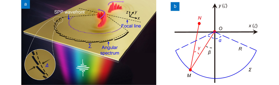
Fig. 1. Schematics of the excitation and spatiotemporal FT modulation of SPP pulses. (a ) Nano-slits in the angular spectrum represented by a reference arc are predesigned in the gold film (200 nm in thickness) on a glass substrate (n =1.515). When illuminated with an angularly dispersed femtosecond pulse, the spatially focused SPP excited by scattering from the slits is temporally modulated through dispersion, while its converging wavefront is spatially modulated by the slits through a displacement ∆ with respect to the reference arc (black dashed curve), thereby realizing both spatial and temporal FT modulation in a SPP focusing structure. (b ) In-plane SPP focusing on metal surface. The field at any point N(x,y) near the focus O(0,0) can be calculated by summing the contributions from all points, e.g., M(ξ, ζ) on a convergent SPP wavefront. γ denotes the angle of inclination of the distance with respect to the normal of the arc ∑; β denotes the angle between MO and the y-axis.
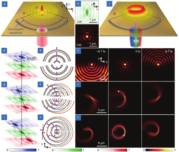
Fig. 2. (a ) Schematic of the spatial FT for a SPP with continuous-wave (CW) incident light. (b ) Spatial distribution of the time-averaged field |E z|2 excited by an 800 nm-wavelength CW source (top) and corresponding temporal wavefront in the SPP focal region (bottom). (c ) Schematic of spatiotemporal FT for a SPP pulse and the angularly dispersed femtosecond laser beam, showing the instantaneous ring-shape formed by the SPP pulses in the focal region. (d ) Spatial distributions of the time-averaged field |E z|2 excited by the 756(blue)/800(green)/850(red)-nm wavelength component of the angularly dispersed femtosecond light with θ =0° in the focal region. (e ) Spatiotemporal evolution of the wavefront of the SPP pulses in the focal region corresponding to (d). The blue/green/red curves mark the equiphase surfaces of the SPP pulses excited by the 756/800/850-nm wavelength components in the focal region, respectively; the black dashed curves marks wavefront of the pulse with its direction of propagation indicated by purple arrows. (f ) The timing diagram for the evolution of the SPP pulse in the focal region corresponding to (e), the time instants being –6.7 fs (before focus), 0 fs (at focus), and 6.7 fs (after focus). (g –i ) and (j –l ) are similar in (d–f) except with θ = 5° and θ = 10°, respectively. All time-averaged fields and timing diagrams are normalized by their respective maximum values. Other settings are R =40 μm, α =180°, τ=10 fs.
Fig. 3. Spatiotemporal FT modulation of the SPP-Airy pulse excited by an arc array of slits [see Fig. 1(a)]. (a ) The time-averaged field |E z|2 of a pulse with centre wavelength 800 nm excited by a y-polarized femtosecond laser beam incident at angle θ =10° to the z-axis but without angular dispersion (left), and an enlargement of field |E z|2 in the focal region (white dashed square) for the 756/800/850-nm wavelength components of the SPP pulses (right). (b ) Same as (a) except with an angular dispersion modulation. The timing diagram for the evolving SPP-Airy pulse in the focal region subject to non-dispersion ((c ) and (d )) and dispersion ((e ) and (f )); ((c) and (e)) present analytical results and ((d) and (f)) present 3D-FDTD simulation results. The green arrow indicates the direction of propagation path of the SPP pulses at the elapsed time given in the top right corner. Other parameters are: R =30 μm, β0 =π/2, p =14, α =180°, τ=10 fs.

Set citation alerts for the article
Please enter your email address
© Copyright 2018-2021 | Chinese Laser Press. All Rights Reserved 沪ICP备15018463号-20