Boundary segmentation based on modified random walks for vascular Doppler optical coherence tomography images

Yong Huang; Chuanchao Wu; Shaoyan Xia; Lu Liu; Shanlin Chen; Dedi Tong; Danni Ai; Jian Yang; Yongtian Wang

doi:10.3788/COL201917.051001

Abstract

Vascular Doppler optical coherence tomography (DOCT) images with weak boundaries are usually difficult for most algorithms to segment. We propose a modified random walk (MRW) algorithm with a novel regularization for the segmentation of DOCT vessel images. Based on MRW, we perform automatic boundary detection of the vascular wall from intensity images and boundary extraction of the blood flowing region from Doppler phase images. Dice, sensitivity, and specificity coefficients were adopted to verify the segmentation performance. The experimental study on DOCT images of the mouse femoral artery showed the effectiveness of our proposed method, yielding three-dimensional visualization and quantitative evaluation of the vessel.

Vessel condition estimation has been a hot topic for a long time. Optical coherence tomography (OCT) is a new imaging modality with high resolution^[1,2], which can combine with the Doppler technique to provide real-time structures and flow images of vessels. Recently, phase images of Doppler OCT (DOCT) were used to monitor the flow status of vessels to assess the surgical outcome of microvascular anastomosis, which is the foundation of plastic and reconstructive surgery^[3]. Driven by the intraoperative application, single vessel segmentation of DOCT images is of great importance.

Due to the strong scattering of blood within the vessel and depth dependent sensitivity roll-off of OCT imaging system, in vivo extra-vascular imaging suffers from low contrast and weak boundaries at the bottom part of the vessel. Currently, segmentation methods of OCT images include four categories. The first uses the intensity images in tissue segmentation, such as the retinal vessels^[4]. The Chan–Vese model is widely used in the second category, such as segmentation of intra-retinal layers^[5]. However, this model depends on the position of the initial contour, and segmentation results are usually influenced by high noises. The third is the machine learning methods. For example, the support-vector machine (SVM) classifier is used in flow segmentation^[6]. Layer-specific edges are segmented by the learning algorithm and trained with the histogram of oriented gradients features, which require learning and training procedures, and thus a large amount of time is inevitable. The fourth is the graph method, which has been widely used in OCT images segmentation^[7], and this segmentation method usually builds an appropriate cost function to distinguish different tissue structures. Therefore, the segmentation problem is transformed into an optimization problem. It takes a long computation time to find the optimal solution.

Grady proposed an effective segmentation algorithm based on random walks^[8], which can detect the weak boundary in images and consume little time. However, for extra-vascular DOCT imaging, direct implementation of the random walks algorithm still has difficulty in detecting the vascular boundary, as strong blood flow scattering induced attenuation, depth dependent sensitivity roll-off, detector saturation effect, and speckle noises have seriously degenerated image contrast and generated weak boundaries at the bottom part of the image.

Sign up for Chinese Optics Letters TOC. Get the latest issue of Chinese Optics Letters delivered right to you！Sign up now

To accurately segment DOCT vessel images from extra-vascular imaging, we proposed a modified random walk (MRW) algorithm, which uses the regularization $D^{2} x$ to obtain a new optimization formulation. This MRW algorithm will create a probability map with superior quality compared with the random walks algorithm, especially for the weak boundary.

The random walks segmentation algorithm originated from the discrete potential theory and electrical circuits^[9]. In Grady’s works, the general image segmentation procedure is as follows: firstly, the small seed points with user-defined labels are given, and then the solution of the Dirichlet integral can quickly determine the probability of the random walking points firstly to reach one of the pre-labeled pixels. Moreover, by assigning each pixel to the label for which the biggest probability is calculated, the image segmentation results are finally determined.

It needs to be pointed out that regularization is used as the Dirichlet integral for obtaining probability map and segmentation results, which are defined as follows: $J (x) = \frac{1}{2} \int_{Ω} {| \nabla x |}^{2} d Ω .$ (1)

However, the use of regularization $\nabla x$ can generate a probability map with the staircase effect^[9], which can cause poor segmentation. To handle this problem, we introduce a new Dirichlet integral $J (x) = \int_{Ω} {| D^{2} x |}^{2} d Ω,$ (2)where $D$ is the differential operator, which denotes gradient operator $\nabla$ . $x$ denotes the probability of a pixel reaching the seed point. According to the Ref. [9], $D^{2}$ represents the combinatorial Laplacian operator, and thus Eq. (2) can become $J (x) = {(L x)}^{2} (L x) = x^{T} (L^{T} L) x = x^{T} Q x,$ (3)where $Q = L^{T} L$ , and $L$ is Laplacian matrix. It may assume that $Q$ and $x$ are ordered without loss of generality. Note that $Q$ is a sparse and semi-definite matrix. Therefore, the set of pixels can be divided into seed and unseeded pixels, and the corresponding transfer probability has two parts $x_{M}, x_{U}$ , respectively. Thus, Eq. (3) can be decomposed into $J [x_{U}] = \frac{1}{2} [\begin{matrix} x_{M}^{T} & x_{U}^{T} \end{matrix}] [\begin{matrix} Q_{M} & B \\ B^{T} & Q_{U} \end{matrix}] [\begin{array}{l} x_{M} \\ x_{U} \end{array}] .$ (4)

Equation (4) takes the derivative of $x_{U}$ and then obtains the following equation: $Q_{U} x_{U} = - B^{T} x_{M} .$ (5)

So, each pixel has its own transition probability. The segmentation result $y$ for two kinds of seeds is also determined through the following equation: $y = {\begin{cases} 1, & x \geq 0.5 \\ 0, & x < 0.5 \end{cases} .$ (6)

From the above process, one can see that the segmentation results depend on the probability map (probability $x$ of every pixel). Thus, the selection of matrix $Q$ is very important. In Eq. (3), Laplacian matrix $L$ is defined as $L_{i, j} = {\begin{cases} d_{i}, & i = j \\ - w_{i j}, & i, j are adjacent \\ 0, & others \end{cases},$ (7)where $d_{i} = \sum_{j} w_{i, j}$ , and $w_{i, j}$ is the weighting value of pixels $i$ and $j$ , which is defined in Ref. [10], and $w_{i j} = \exp [- β {(g_{i} - g_{j})}^{2}] [1 - \exp (- α z)],$ (8)where $α (> 0)$ is the estimated attenuation coefficient. $β$ is a free parameter. In this work, the $β$ value is 90. $g_{i}$ and $g_{j}$ are image intensity values of pixels $i$ and $j$ . $z$ denotes the pixel position in the vertical direction.

Due to the imaging depth limitation of the DOCT system, there is a low contrast in the position of a large $z$ value, such as DOCT images of Fig. 1(a). To increase the success of the edge extraction at the low contrast position of DOCT images, Eq. (8) uses $1 - \exp (- α z)$ to compensate the intensity value caused by the DOCT structure image signal attenuation. In general, the DOCT structure image suffers from depth dependent attenuation; thus, the attenuated signal $I$ is given by $I = I_{0} \exp (- α z),$ (9)where $I_{0}$ is the initial intensity. To realize the automatic estimation of the attenuation coefficient $α$ for each image, we use Eq. (9) as the prediction model to get the coefficients automatically.

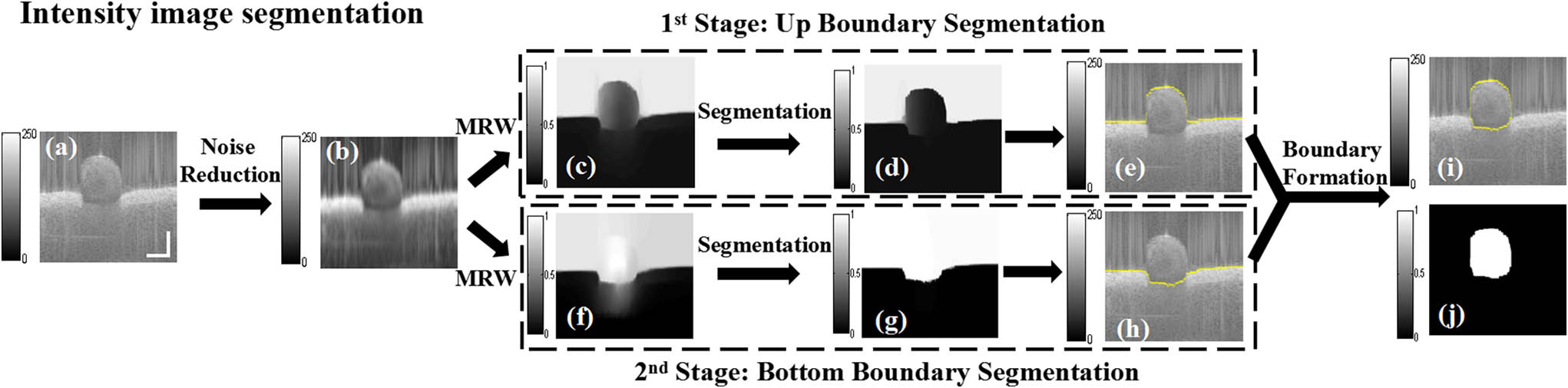
Figure 1.MRW algorithm segmentation procedure of intensity image. First stage shows the process of upper boundary segmentation. Second stage shows the process of bottom boundary segmentation. Then, they are combined to create an intact boundary mask (scale bar: 500 μm).

The whole segmentation process of the MRW algorithm involves two parts: boundary detection of the vessel wall from the intensity image and boundary exaction of the blood flow region from the phase image. Note that the boundary extraction of the vessel wall is divided into two stages, where the MRW algorithm is applied to detect the upper and bottom boundaries of the vessel wall, respectively.

The segmentation object is mouse artery images of the Fourier domain OCT (FDOCT) system^[11]. To reduce the noise influence of Fig. 1(a), we use the sparse and representations method^[12] to address the noise, as shown in Fig. 1(b). However, the filtered image still shows blurred edges, especially for the bottom boundary of the blood vessel. If the filtered image is used as the segmentation object, low contrast between the boundary and background area will still cause poor segmentation results. To improve the segmentation accuracy, we use the probability map [see Fig. 1(c) or 1(f)] of the MRW algorithm as the segmentation object, which can provide a higher contrast image than the original image [Fig. 1(a)] and filtered image [Fig. 1(b)].

During the MRW process, two kinds of seeds are selected for the MRW algorithm. It is important to select the seed point’s position in the intensity image, especially for the weak vessel boundary. Furthermore, seed points are two classes of pixels, instead of only two pixels. For the first segmentation stage of the vessel wall, the first kind of seed points is located at the top of the intensity image [see the green line in Fig. 2(a)], and the second kind of seed points is distributed at the bottom of the intensity image [see the blue line in Fig. 2(a)]. Then, by using the MRW algorithm, the probability map is generated in Fig. 1(c). Finally, the upper boundary can be well detected [see Fig. 1(d)].

Figure 2.Selection of seed points in the segmentation stages for OCT intensity image. (a) Two kinds of seeds are selected for the upper boundary segmentation in the first stage, marked by green and blue lines, respectively. (b) Two kinds of seeds are selected for the bottom boundary segmentation in the second stage, marked by green and blue lines, respectively (scale bar: 500 μm).

In the second stage of the vessel wall process, the selection of seed points still includes two classes. The seed points of the first class derive from the upper boundary [see the green line in Fig. 2(b)]. The seed points of the second class are located near the bottom of the intensity image [see the blue line in Fig. 2(b)]. Under these two classes of seed points and the MRW algorithm, a new probability map of the intensity image is created, as shown in Fig. 1(f). Then, this new probability map once again is used as the segmentation object, and the MRW algorithm adopts seed points in the position of Fig. 2(b) to detect the bottom boundary, as shown in Fig. 1(g). Finally, segmentation lines of the probability map in Figs. 1(e) and 1(h) were mapped to the intensity image of Fig. 1(a) after using the morphological operation (open operation and select maximum connected domain) for the region between the two boundaries where the vascular boundary [Fig. 1(i)] and segmentation mask [Fig. 1(j)] are obtained. With these processes, the boundary detection of the vessel wall is completed.

The phase image [see Fig. 3(b)] shows a lot of random noise. It makes segmentation difficult. The mask [see Fig. 3(a)] from the intensity segmentation process can remove the background interference of the phase image, which makes the segmentation of the phase image easy, as shown in Fig. 3(c). It is apparent that there is no Doppler signal between the vessel wall and blood flow. Thus, in the segmentation process of the phase image, we treat the pixels satisfying the simple threshold condition $| φ | \geq 2.5$ (where $φ$ is the phase value) as one kind of the seeds. In addition, the other kind of seeds is the pixels located in the segmentation line of the intensity image. Similarly, by using the MRW algorithm, the probability map of the blood flow region is obtained, as shown in Fig. 3(d). Then, the segmentation line is extracted [see Fig. 3(e)]. Hence, boundaries of the vessel wall and blood flow region are indicated in Fig. 3(f).

Figure 3.Segmentation procedure of the phase image. We combined phase image with a boundary mask to remove the background, and then made use of the threshold condition to get the blood flow region (scale bar: 500 μm).

In the MRW process, we use the regularization $D^{2} x$ to optimize the algorithm. To illustrate the MRW advantage, we use $\nabla x$ and $D^{2} x$ as two regularizations to segment intensity images. Figure 4 shows the comparison results of the second segmentation stage in the intensity images [from Figs. 1(f) to 1(g)]. Figures 4(a) and 4(c) are probability maps after using the regularizations of $\nabla x$ and $D^{2} x$ , respectively. Figures 4(b) and 4(d) are corresponding segmentation results. From the comparison, one can see that the probability map of regularizations $\nabla x$ has the staircase effect in vessel tissue. For the two classifications, the critical point of probability is $x = 0.5$ , so the staircase effect of Fig. 4(a) causes the wrong segmentation result [see Fig. 4(b)]. On the contrary, Fig. 4(c) shows that the regularization $D^{2} x$ has a smoother probability map than $\nabla x$ , and thus the corresponding segmentation result becomes more accurate [see Fig. 4(d)]. Therefore, the MRW algorithm can provide a more suitable probability map for the weak boundary accurate segmentation. We assume the reason might be that the combinatorial Laplacian operator as a second-order operation reflects pixel intensity changes in more locations compared to the first-order gradient operator, which only reflects the pixel intensity changes in adjacent positions.

Figure 4.Probability map and corresponding segmentation results using different regularization. (a) Probability map using the regularization $\nabla x$ . (b) Segmentation result of (a). (c) Probability map using the regularization $D^{2} x$ . (d) Segmentation result of (c) (scale bar: 500 μm).

To verify the validity of the MRW algorithm, we also applied MRW to segment the mouse artery images from the FDOCT system^[11], where each B-scan image consisted of 1000 A scans, and each C scan consisted of 250 B scans. To exhibit the segmentation capability in the different blood flow regions, we select four groups of OCT images from the various positions of mouse blood vessels, as shown in Fig. 5. It shows the phase images from a healthy vessel [see Fig. 5(a-2)] and three group blood vessels [see Figs. 5(b-2)–5(d-2)] with different seriousness of arteriosclerosis, and corresponding structure images of the vessels are Figs. 5(a-1)–5(d-1). The weak boundary of the vessel bottom can be successfully detected in the four group intensity images. Under the mask from the intensity image, the phase image with background removal is segmented, and accuracy and the boundary of the blood flow region are well captured in Figs. 5(a-2)–5(d-2).

Figure 5.Segmentation results of different OCT frames. (a-1)–(d-1) OCT intensity images of frames 1, 65, 131, 192, and segmentation results, respectively. (a-2)–(d-2) OCT phase images of frames 1, 65, 131, 192, and segmentation results, respectively (scale bar: 500 μm).

To further evaluate the performance of MRW algorithm in segmentation of DOCT blood vessel images, we compared our segmentation results with ground truth of the manual segmentation results. The quantitative evaluation parameters contain the Dice coefficient (DC), sensitivity coefficient (SNC), and specificity coefficient (SPC)^[13], which are computed as follows: $DC = \frac{2 TP}{2 TP + FP + FN}, SNC = \frac{TP}{TP + FN}, SPC = \frac{TN}{TN + FP},$ (10)where TP is true positive, FP is false positive, FN is false negative, and TN is true negative. DC is the ratio of the intersection area between the segmented region and the manual region. SNC refers to how many pixels in the manual region are correctly segmented, and SPC measures how many pixels are outside the manual region.

The evaluation parameters are computed as shown in Table 1. For this process, it was conducted through MATLAB R2013 in a computer with the Intel ^®Core™ i7-4790 processer at 3.6 GHz and 8 GB random access memory (RAM). The values of DC and SNC are above 90%. All of the values of SPC are nearly 100%; thus, these values indicate that almost no pixels fall to the outside of manual regions. It illustrates that the segmentation results are basically consistent with the manual process results.

Group	Frame 1		Frame 65		Frame 131		Frame 192
Image Type	Intensity	Phase	Intensity	Phase	Intensity	Phase	Intensity	Phase
DC (%)	96.60	95.66	96.55	94.98	97.11	92.31	96.12	95.13
SNC (%)	98.79	92.54	97.04	91.01	98.95	90.97	97.96	92.08
SPC (%)	99.46	99.93	99.53	99.96	99.42	99.61	99.39	99.88

Table 1. Evaluation Parameter Comparison Between Segmentation Results and Ground Truth

View all Tables

In addition, we completed the segmentation task of 250 frame DOCT images automatically. These two-dimensional (2D) images are used to reconstruct the three-dimensional (3D) vessel wall with ImageJ software after they are registered by the sub-pixel image registration algorithm^[14,15], as shown in Fig. 6. Figures 6(a) and 6(b) are the upper and bottom parts of the vessel wall, respectively. From 3D visualization, we can clearly see that there is thrombosis existence at positions 1 and 2, which indicates the severity of vessel condition. It is helpful to evaluate vessel stenosis and show the thrombotic morphology intuitively.

Figure 6.3D reconstruction of the vessel. (a) The upper part of the blood vessel. (b) The bottom part of the blood vessel. The arrows point at the thrombosis position.

Quantitative analysis was performed after segmentation to help with the objective evaluation of the surgical outcome. We analyzed the blood flow area and blood vessel radius along the blood flow axis based on the segmentation results of 250 frame DOCT images. Thrombosis and stenosis will generate a small blood flow area that is detrimental to long term success. Figure 7(a) shows the inner blood flowing area variation along the vessel flow axis. It clearly shows that the blood flow area becomes narrower when thrombosis occurs near the position of 0.4 and 0.75 mm. The mean radius of the blood flow area in 10 angular directions at one cross-sectional image and their standard deviation are shown in Fig. 7(b). Along the blood flow direction, the variation of vessel radius is large. For positions with thrombus, the inner radius of the blood vessel becomes significantly smaller. In addition, a large radius standard deviation value is more prone to turbulence generation. Later, these physical parameters can be fed into the computational fluid dynamics (CFD) model to simulate the blood flow of the vessel and analyze wall shear stress at the vessel^[16], especially for arteries with serious stenosis or thrombosis^[17], in the future work.

Figure 7.(a) Blood flow area variation along the blood flow axis. (b) Blood vessel radius variation along the blood flow axis.

In this present work, we developed an MRW method with a new regularization $D^{2} x$ for extra-vascular DOCT image segmentation, which improves the segmentation results of weak boundaries. Using this method, we automatically completed the segmentation process of 250 frame DOCT mouse artery vessel images. Moreover, utilizing these segmentation results, 3D reconstruction of the vessel, and quantitative analysis of the blood flow area and the radius variation were completed. We believe this work will contribute to the construction of objective methods for the anastomosis surgery assessment.

References

[1] D. Huang, E. A. Swanson, C. P. Lin, J. S. Schuman, W. G. Stinson, W. Chang, M. R. Hee, T. Flotte, K. Gregory, C. A. Puliafito, J. G. Fujimoto. Science, 254, 1178(1991).

[2] R. Dsouza, H. Subhash, K. Neuhaus, P. M. McNamara, J. Hogan, C. Wilson, M. J. Leahy. Chin. Opt. Lett., 15, 090007(2017).

[3] Y. Huang, Z. Ibrahim, D. Tong, S. Zhu, Q. Mao, J. Pang, W. P. Andree Lee, G. Brandacher, J. U. Kang. J. Biomed. Opt., 18, 111404(2013).

[4] C. Kharmyssov, M. W. L. Ko, J. R. Kim. Chin. Opt. Lett., 17, 011701(2019).

[5] A. Yazdanpanah, G. Hamarneh, B. R. Smith, M. V. Sarunic. IEEE Trans. Med. Imaging, 30, 484(2011).

[6] A. S. G. Singh, T. Schmoll, R. A. Leitgeb. Biomed. Opt. Express, 2, 1328(2011).

[7] D. Kaba, Y. Wang, C. Wang, X. Liu, H. Zhu, A. G. Salazar-Gonzalez, Y. Li. Opt. Express, 23, 7366(2015).

[8] L. Grady. IEEE Trans. Pattern Anal. Mach. Intell., 28, 1768(2006).

[9] L. Grady, J. R. Polimeni. Discrete Calculus: Applied Analysis on Graphs for Computational Science(2010).

[10] A. Karamalis, W. Wein, T. Klein, N. Navab. Med. Image Anal., 16, 1101(2012).

[11] Y. Huang, G. J. Furtmüller, D. Tong, S. Zhu, W. P. A. Lee, G. Brandacher, J. U. Kang. PLoS ONE, 9, e114215(2014).