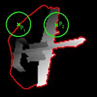
Fig. 1. Explanation of how to adaptively determine the weight coefficient of global fitting term

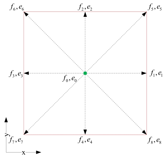
Fig. 2. Spatial structure of the D2Q9 LBM lattic

Fig. 3. The flowchart the proposed GPU accelerated segmentation model

Fig. 4. Segmentation comparisons of C-V model, K-means model, PCNN model and our method on five laser radar range images.The first row: Input images along with initial contours,the second row: C-V model, the third row: K-means model,the fourth row: PCNN model;the fifth row: our model.

Fig. 5. The segmentation results on several sampleimagesof the PASCAL VOC 2012 dataset.The first column shows the input images along with initial contours, and the second to fifth columns is the segmentation results by using C-V, K-means, PCNNand our models respectively

Fig. 6. Quantitative evaluation results of four different comparison algorithms on VOC 2012 dataset.The sub-graphs (a) and (b) are the statistical distributions of the two metrics JS and DSC, respectively. Any single boxplot corresponds to the comprehensive response results of an algorithm participating in the comparison on the VOC 2012 dataset.

Fig. 7. Segmentation comparisons of our model with LBF model on an infrared human body image under three different initializations.The first row: Input images along with initial contours; the second row: Final segmentation results of LBF model; the third row:Final segmentation results of our model

Fig. 8. Segmentation comparisons of our model with LBF model on an infrared pig image under three different initializations.The first row: Input images along with initial contours; the second row: Final segmentation results of LBF model; the third to fifth rows: Three intermediate results of our model; the sixth row:Final segmentation results of our model

Fig. 9. The statistical results corresponding to the evolution process shown in Fig. 8.The first row is the global mean image at convergence state, the second to third rows are the numerical distribution images of e1 and e2at convergence state, the fourth row is the energy variation curve with respect to the evolution time, and the fifth row is the evolution process of three-dimensional stacking form.

Fig. 10. A set of experiments to test the rapidity of evolution process.The first row is the input images along with initial curves, the second to fourth rows are three intermediate results of the evolution process, and the fifth row is the final segmentation results.

Fig. 11. The statistical results corresponding to the experimental process shown in Fig. 10.The first row is the global mean image at convergence state, the second to third rows are the numerical distribution images of e1 and e2at convergence state, the fourth row is the energy variation curve with respect to the evolution time, and the fifth row is the evolution process of three-dimensional stacking form.

Fig. 12. The test image used to verify the effect of adaptive weighting coefficient on segmentation results and the different expressions of adaptive weighting coefficients. (a) Example image with two sampling points A and B; (b) The image representation form of the adaptive weighting matrix and the coefficient values corresponding to the two sampling points in (a); (c) The 3D surface representation of adaptive weighting coefficient matrix.

Fig. 13. A verification experiment used to test the effect of adaptive weighting coefficients on segmentation results (a) Input image along with initial contour; (b) Segmentation result when regional term plays a dominant role; (c) Segmentation result when edge term plays a dominant role; (d) Segmentation result returned by the proposed model.

Fig. 14. The relationship between function δεnewx and its independent variable x under different parameter ε

Table 1. Corresponding forms of τ and F in D2Q9 LBM equation for level set methods

Table 2. Segmentation metrics for the five images in Fig. 4numberedin order from left to right

Table 3. Comparisons of speed metrics of evolution process for the three images in Fig. 10 numbered in order from left to right