GPU accelerated level set model solving by lattice boltzmann method with application to image segmentation

Wen-Jun SHI; Deng-Wei WANG; Wan-Suo LIU; Da-Gang JIANG

doi:10.11972/j.issn.1001-9014.2021.01.016

Abstract

A novel Graphics Processing Units (GPU) accelerated level set model which organically combines the global fitting energy and the local fitting energy from different models and the weighting coefficient of the global fitting term can be adaptively adjusted, is proposed to image segmentation. The proposed model can efficiently segment images with intensity inhomogeneity regardless of where the initial contour lies in the image. In its numerical implementation, an efficient numerical scheme called Lattice Boltzmann Method (LBM) is used to break the restrictions on time step. In addition, the proposed LBM is implemented by using a NVIDIA GPU to fully utilize the characteristics of LBM method with high parallelism. The extensive and promising experimental results from synthetic and real images demonstrate the effectiveness and efficiency of the proposed method.In addition, the factors that can have a key impact on segmentation performance are also analyzed in depth.

Keywords

graphics processing unit Intensity inhomogeneity Lattice Boltzmann method level set method segmentation

Introduction

Image segmentation is a fundamental task in many image processing and computer vision applications. Due to the presence of noise，low contrast，and intensity inhomogeneity，it is still a difficult problem in majority of applications.Image segmentation techniques have been extensively studied over the past few decades. A well-established class of methods is active contour models^［1-3］，which are based on the theory of surface evolution and geometric flows，have been deeply studied and successfully used in image processing. The level set method（LSM）proposed by Osher and Sethian^［4］ is widely used in solving the problems of surface evolution. Later，geometric flows were unified into the classic energy minimization formulations for image segmentation^［5-8］. Generally speaking，the existing active contour models can be categorized into two types：edge-based models^［9-10］ and region-based models^［11-12］. The edge-based models use the gradient information of the image to construct the driving force required for the evolution process. When the input image has a sharp gradient，such models can indeed output high-quality segmentation results. However，they may suffer from some terrible problems such as poor robustness to noise interference，highly sensitive to initialization，edge leakage，and easy to fall into local minimum. Contrary to the edge-based models，the region-based active contour models use the regional statistical information from inside and outside of the evolution contour to construct the driving force to guide the whole level set evolution process. Compared with the edge-based models，region-based models have the following obvious advantages：First，region-based models have more freedom in terms of the contour initialization，i.e.，the initial contour can be located anywhere in the image coordinate system，and the exterior and interior contours can be detected simultaneously. Second，they are very insensitive to noise and can efficiently segment the images with weak edges or even without edges. One of the most successful region-based models is the Chan-Vese（C-V）model ^［11］，which has been widely used in binary phase segmentation with the assumption that each image region is statistically homogeneous. However，the C-V models fail to segment the images with intensity inhomogeneity.

In order to overcome the segmentation difficulty caused by the intensity inhomogeneity，some local region-based segmentation models^［13-15］ had been proposed. These methods generally believe that the images with intensity inhomogeneity satisfy the assumption of homogeneity within a very small local region，that is，within a sufficiently small local image region，we can assume that the intensity of the image is approximately statistically uniform.Thus，by fitting the given image in the sense of local region rather than global region，they can segment the images with intensity inhomogeneity. For example，in Ref.［13］，the entire target boundary is obtained by minimizing the local binary fitting（LBF）energy. Since the LBF model makes full use of the local region information，it achieves good segmentation performance in segment inhomogeneous images. However，like most existing active contour models，the LBFmodel is also very sensitive to contour initialization，which restricts its application range to some extent.

In addition，over the past few years，the GPU has been proposed as a general-purpose computing architecture. As the simple increase in the clock speed will push the transistors to thermal limits，the multi-core technology has become an obvious solution to enhance the computing performance. In this context，The GPU has been recognized as one of the most promising techniques to accelerate scientific computations. The GPU architecture favors dense data and local computations because the communications between microprocessor is time consuming.

In order to overcome the problems mentioned above and take into account the promotion role of GPU in terms of computation，in this paper，we propose a new GPU accelerated region-based active contour model under variational level set framework. Firstly，based on the two models of C-V and LBF，we construct a hybrid level set model，which integrates the global fitting energy used in C-V model and the local fitting energy used in LBF model and the weighting coefficient of the global fitting term can be adaptively adjusted. The proposed model can not only segment inhomogeneous and weak-edge targets，but also make evolution process insensitive to contour initialization，i.e.，our model inherits the advantages of the two models of C-V and LBF，while overcoming their respective shortcomings. Secondly，in its numerical implementation，we adopt the LBM method，which can break the restrictions of the traditional implementation methods on time step. Compared with the traditional schemes，the LBM strategy can further shorten the time consumption of the evolution process，thus allows the level set to quickly reach the true target location. Thirdly，the proposed level set model is computed by using a NVIDIA GPU to fully utilize the characteristics of LBM method of high parallelism.

The remainder of this paper is organized as follows：Section 2 is a brief description of the classical C-V and LBF models which are background knowledge directly related to the proposed model. Section 3 presents the formulation and implementation of the proposed model. Section 4 validates the proposed model by extensive experiments and discussions on synthetic and real images. Last，conclusions are drawn in section 5.

1.1　C-V model

When the classical active contour models perform image segmentation tasks，their external energy terms are usually based on the local gradient information of the image. Such external energy terms can perform excellently when the gradient of the image is very obvious. However，for those images whose contours are either smooth or cannot be defined by gradient，the aforementioned energy terms will undoubtedly encounter great difficulties. In order to solve this problem effectively，Chan and Vese^［11］ proposed a novel region-based active contour model（usually referred to as C-V model）based on the simplified Mumford-Shah model. Its energy functional definition is as follows：

\begin{array}{l} E^{C V} (ϕ) = λ_{1}^{C V} {\int_{Ω} (I (x) - M_{i n})}^{2} H (ϕ (x)) d x + \\ λ_{2}^{C V} {\int_{Ω} (I (x) - M_{o u t})}^{2} (1 - H (ϕ (x))) d x + \\ μ \cdot \int_{Ω} δ (ϕ (x)) |\nabla ϕ (x)| d x + ν \cdot \int_{Ω} H (ϕ (x)) d x \end{array}

,（1）

where $H (\cdot)$ and $δ (\cdot)$ are one-dimensional Heaviside and Dirac functions. This minimization problem is solved by deducing the associatedEuler-Lagrange equations and updating the level set function $ϕ$ by the gradient descent method（with $ϕ (0, x) = ϕ_{0} (x)$ defining the initial contour）：

\frac{\partial ϕ}{\partial t} = δ (ϕ) [μ d i v (\frac{\nabla ϕ}{|\nabla ϕ|}) - ν - λ_{1}^{C V} {(I - M_{i n})}^{2} + λ_{2}^{C V} {(I - M_{o u t})}^{2}]

,（2）

where $M_{i n}$ and $M_{o u t}$ can be updated iteratively by

\{\begin{array}{l} M_{i n} (ϕ) = \frac{\int_{Ω} I (x) H (ϕ (x)) d x}{\int_{Ω} H (ϕ (x)) d x d y} \\ M_{o u t} (ϕ) = \frac{\int_{Ω} I (x) (1 - H (ϕ (x))) d x}{\int_{Ω} (1 - H (ϕ (x))) d x} \end{array}

,（3）

and $- λ_{1}^{C V} {(I - M_{i n})}^{2} + λ_{2}^{C V} {(I - M_{o u t})}^{2}$ is the global image fitting force，which uses the global image information of the input image to guide the evolution of level set model. As a representative region information-based level set segmentation model，the C-V model has an important characteristic，i.e.，its evolution is not sensitive to the initial position of the curve. However，when the intensity of the image is not homogeneous，the difference between the two means（ $M_{i n}$ and $M_{o u t}$ ）and the real image data will be very large，this phenomenon will inevitably lead the C-V model to be difficult to give an ideal segmentation result.

1.2　LBF MODEL

In order to extend the application range of the level set model to the field of inhomogeneous image segmentation applications，Li et al. constructed a region-based active contour model based on the local region statistical information of the image. It first defines a local energy function with the following expression for each pixel x on the image plane：

\begin{array}{l} E_{x} = λ_{1}^{L B F} \int_{i n s i d e (C)} K_{σ} (x - y) |I (y) - f_{1} {(x)}^{2}| d y d x + \\ λ_{2}^{L B F} \int_{o u t s i d e (C)} K_{σ} (x - y) |I (y) - f_{2} {(x)}^{2}| d y d x \end{array}

,（4）

where $I$ is the image data to be segmented， $C$ is a closed contour on the image plane， $λ_{1}^{L B F}$ and $λ_{2}^{L B F}$ are two control constants for balancing the forces inside and outside the contour $C$ ， $K_{σ}$ is a Gaussian window function（the localization effect of the LBF model is exactly caused by this window function）with standard deviation $σ$ ， $f_{1} (x)$ and $f_{2} (x)$ are fitting values of two sub-regions divided by the contour $C$ （the divided object is the local region centered at the current pixel $x$ ）.

Then，by integrating the aforementioned energy function over the entire image region，the overall target functional of the LBF model in form of level set formulation can be generated as follows：

\begin{array}{l} E^{L B F} = \int_{Ω} E_{x} (ϕ, f_{1} (x), f_{2} (x)) d x \\ = λ_{1}^{L B F} \int_{Ω} [\int_{Ω} K_{σ} (x - y) {|I (y) - f_{1} (x)|}^{2} H (ϕ (y)) d y] d x \\ + λ_{2}^{L B F} \int_{Ω} [\int_{Ω} K_{σ} (x - y) {|I (y) - f_{2} (x)|}^{2} (1 - H (ϕ (y))) d y] d x \end{array}

,（5）

where $ϕ (\cdot)$ is the level set function and $H (\cdot)$ is the Heaviside function. Minimizing the energy functional $E^{L B F}$ with respect to $ϕ$ by using the calculus of variation and the steepest descent method，we can easily deduce the corresponding gradient descent flow as：

\frac{\partial ϕ}{\partial t} = - δ (ϕ) (λ_{1}^{L B F} e_{1} - λ_{2}^{L B F} e_{2})

,（6）

$e_{1}$ and $e_{2}$ in Eq.（6） are defined as：

\{\begin{array}{l} e_{1} (x) = \int_{Ω} K_{σ} (y - x) {|I (x) - f_{1} (y)|}^{2} d y \\ e_{2} (x) = \int_{Ω} K_{σ} (y - x) {|I (x) - f_{2} (y)|}^{2} d y \end{array}

,（7）

with

\{\begin{array}{l} f_{1} (x) = \frac{K_{σ} * [H_{ε} (ϕ) I (x)]}{K_{σ} * H_{ε} (ϕ)} \\ f_{2} (x) = \frac{K_{σ} * [1 - H_{ε} (ϕ) I (x)]}{K_{σ} * [1 - H_{ε} (ϕ)]} \end{array}

.（8）

In the above equations，we actually use the regularized versions of Heaviside function $H (\cdot)$ and Dirac function $δ (\cdot)$ which are expressed as follows：

\{\begin{array}{l} H_{ε} (z) = \frac{1}{2} [1 + \frac{2}{π} a r c t a n (\frac{z}{ε})] \\ δ_{ε} (z) = \frac{1}{π} \cdot \frac{ε}{ε^{2} + z^{2}}, z \in R \end{array}

.（9）

The parameter $ε$ affects the profile of $δ_{ε} (ϕ)$ . A bigger $ε$ will cause a broader profile，which will expand the capture scope but decrease the accuracy of the final contour.

In actual calculation，the construction process of the local binary image $(λ_{1}^{L B F} e_{1} - λ_{2}^{L B F} e_{2})$ is based on all the pixels in a local Gaussian window，this localization property is the real reason for the LBF model to be able to segment non-homogenous images.However，when the contour is located at a certain location where $λ_{1}^{L B F} e_{1} = λ_{2}^{L B F} e_{2}$ ，the local image fitting force will be zero，which leads to the evolution process be trapped into certain local minima，thus the segmentation result has a strong correlation with the initial position of the curve.

2　The proposed method

2.1　Our model and its variational level set formulation

For the segmenting level set function $ϕ$ of an image，we define its local fitting energy as：

\begin{array}{l} E^{l o c a l} (ϕ) = λ_{1}^{C V} \int_{Ω} [\int_{Ω} K_{σ} (x - y) {|I (y) - f_{1} (x)|}^{2} H (ϕ (y)) d y] d x + \\ λ_{2}^{C V} \int_{Ω} [\int_{Ω} K_{σ} (x - y) {|I (y) - f_{2} (x)|}^{2} (1 - H (ϕ (y))) d y] d x \end{array}

.（10）

At the same time，its corresponding global fitting energy is defined as the following form：

\begin{array}{l} E^{g l o b a l} (ϕ) = λ_{1}^{L B F} {\int_{Ω} (I (x) - M_{i n})}^{2} H (ϕ (x)) d x + \\ λ_{2}^{L B F} {\int_{Ω} (I (x) - M_{o u t})}^{2} (1 - H (ϕ (x))) d x \end{array}

.（11）

They come from the two models of C-V and LBF，respectively.By combining these two energy terms，we propose the new energy functional as follows：

E (ϕ) = E^{l o c a l} (ϕ) + w \cdot E^{g l o b a l} (ϕ)

,（12）

where $w$ is a weight control parameter and its value varies with image coordinates.

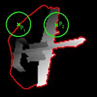
To get better segmentation results，we need to make a reasonable combination of $E^{l o c a l} (ϕ)$ and $E^{g l o b a l} (ϕ)$ in Eq.（12）. The key point is how to adaptively determine the weight coefficient $w$ of the auxiliary global fitting energy term.In regions far from the true target boundaries，such as point $p_{1}$ in Fig. 1，where the intensity distribution is nearly homogeneous，the fitting values $f_{1}$ and $f_{2}$ obtained by local fitting process are almost identical，which means that within this type of regions， $f_{1}$ and $f_{2}$ cannot correctly reflect real background information and foreground targets.The reason is that the processing flow only takes into account the local information. However，in such regions，local information is not sufficient for the true background and foreground description task. In view of this，we need to increase the weight coefficient of the global fitting term so that the active contour can towards right direction under the driving of global fitting energy. Conversely，within the regions close to the true target boundaries，for example，point $p_{2}$ in Fig. 1. At this time，the foreground $f_{1}$ and background $f_{2}$ obtained by local fitting process can correctly reflect the distributions of foreground and background.When the image has an inhomogeneous intensity distribution， $M_{i n}$ and $M_{o u t}$ obtained by global fitting process may seriously deviate from the real foreground and background，and the existence of global fitting term will affect the accuracy of segmentation.As a result，in such regions，we need to reduce the weight coefficient of global fitting energy to ensure the accuracy of segmentation output.

Figure 1.Explanation of how to adaptively determine the weight coefficient of global fitting term

Based on the above analysis，we should adaptively generate the weighting coefficient of global fitting term according to the image region in which the active contour is located，i.e.，in a region where intensity changes smoothly，a smaller value needs to be taken，while in a region where intensity changes greatly，it is necessary to take a larger value. To match this requirement，we define the following local contrast factor corresponding to a local window：

L C R_{N} = \frac{V_{m a x} - V_{m i n}}{L}

,（13）

where $N$ is used to mark the size of the local window， $V_{m a x}$ and $V_{m i n}$ are the maximum and minimum intensity values of the local window，respectively， $L$ is the intensity level of image，and for grayscale images，its value is 255. Obviously，the value range of $L C R_{N}$ is $[0,1]$ . At the physical meaning level，it reflects how fast the intensity changes in a local region，which have smaller values in the smooth regions and bigger values in the regions close to targets boundaries. In view of this，we define the weight coefficient as the following functional form：

w = κ \cdot m e a n (L C R_{N}) . (1 - L C R_{N})

,（14）

where $κ$ is a constant parameter， $m e a n (L C R_{N})$ is the average value of $L C R_{N}$ over the entire image region，which reflects the overall contrast of the image. For images with strong overall contrast，they must have a clear foreground and background，so we can increase the weight coefficient on the whole. $(1 - L C R_{N})$ can adaptively adjust the weight coefficient of global term in all local regions，making it smaller in regions with high local contrast ratio and larger in regions with low local contrast ratio.

For more accurate computation involving the level set function and its evolution，we need to regularize the level set function by penalizing its deviation from a signed distance function^［16］，characterized by the following energy functional：

P (ϕ) = \int \frac{1}{2} {(|\nabla ϕ (x)| - 1)}^{2} d x

.（15）

As in typical level set methods，we need to regularize the zero level set by penalizing its length to derive a smooth contour which is as short as possible during evolution：

L (ϕ) = \int |\nabla H (ϕ (x))| d x

.（16）

In summary，we can express the total energy functional as the following：

E^{o u r} = E + μ \cdot P (ϕ) + ν \cdot L (ϕ)

,（17）

where $μ$ and $ν$ are control parameters to balance the contribution of the corresponding energy term.

Keeping $M_{i n}$ and $M_{o u t}$ fixed，and minimizing the entire energy functional Energy with respect to $ϕ$ ，we deduce the associated Euler-Lagrange equation for $ϕ$ as follows：

\begin{array}{l} \frac{\partial ϕ}{\partial t} = δ_{ε} (ϕ) (- λ_{1}^{C V} {(I - M_{i n})}^{2} + λ_{2}^{C V} {(I - M_{o u t})}^{2}) - \\ w \cdot δ_{ε} (ϕ) (λ_{1}^{L B F} e_{1} - λ_{2}^{L B F} e_{2}) + \\ μ (Δ ϕ - d i v (\frac{\nabla ϕ}{|\nabla ϕ|})) + ν δ_{ε} (ϕ) d i v (\frac{\nabla ϕ}{|\nabla ϕ|}) \end{array}

,（18）

where $M_{i n}$ ， $M_{o u t}$ ， $e_{1}$ and $e_{2}$ are formulated by expressions（3），and（7），respectively.

The new hybrid fitting energy is a weighted linear combination of the global image fitting force from the C-V model and the local binary fitting force from the LBF model. The advantages of this weighted combined form of image fitting energy are as follows：The global image fitting force component makes the combined model insensitive to the initial position of the curve，and the local binary fitting force component makes the combined model can segment the images with intensity inhomogeneity. We combine these two forces together with the control parameter $w$ so that the new hybrid model can have the advantages of the C-V model and the LBF model. Therefore，the proposed model can effectively deal with the intensity inhomogeneity，regardless of where the initial contour lies in the image.

2.2　The implementation of the proposed model

2.2.1　The reason for the high computational complexity of traditional level set methods

The traditional level set methods usually need to spend more iterative times（corresponding to a higher time consumption）to segment an image，which is unacceptable for image data-based real time applications or mass image data processing problems. The following reason leads to this high computational complexity phenomenon：An explicit scheme is the most popular way for solving Eq.（18），but due to the Courant-Friedreichs-Lewy（CFL）^［17］ condition which asserts that the numerical waves should propagate at least as fast as the physical waves，so the curve can only move a small distance in each iteration，it requires very small time step and if the curve is not near the edge of interested object，the curve may take a long time to reach the final position.

2.2.2　Lattice Boltzmann Method for breaking the restrictions on time step

The CFL condition limits the time step of the traditional numerical solution of the level set equation，which leads to the increase of the number of iterations in the evolution process. Under the finite difference framework，the process needs to approximate the continuous PDE to a discrete form，while LBM^［18］derives a continuous PDE which has the same form of the level set equation from a discrete form. Since the time step is not strongly restricted and highly parallelizable，LBM is a fast numerical solution of the level set equation.

LBM is proposed as a computational fluid dynamics（CFD）method for fluid modeling^［19］. Instead of solving the Navier-Stokes equations，the discrete boltzmann equation is solved to simulate the flow of the Newtonian fluid by collision models such as Bhatnagar-Gross-Krook（BGK）^［20-21］.

In this paper，we use the D2Q9（2D with 8 links with its neighbors and one link for the cell itself）LBM lattice structure. Fig. 2 shows a typical D2Q9 model.

Figure 2.Spatial structure of the D2Q9 LBM lattic

The evolution equation of LBM can be written as

\begin{array}{l} f_{i} (\vec{r} + \vec{e_{i}} Δ t, t + Δ t) = f_{i} (\vec{r}, t) + \frac{1}{τ} [f_{i}^{e q} (\vec{r}, t) - f_{i} (\vec{r}, t)] \\ + \frac{D}{b c^{2}} \cdot \vec{F} \cdot \vec{e_{i}} \end{array}

,（19）

where $\vec{e_{i}}$ is the velocity vector of a given link $i$ ， $f_{i} (\vec{r}, t)$ the distribution of the particle that moves along that link， $t$ the time， $Δ t$ the time step， $\vec{r}$ the position of the cell， $\vec{F}$ the body force， $D$ the grid dimension， $b$ the link at each grid point and $c$ the length of each link which is set to 1 in this paper. The parameter $τ$ represents the relaxation time determining the kinematic viscosity in Navier-Stokes equations，and $f_{i}^{e q}$ is the local equilibrium particle distribution which has the following form.

f_{i}^{e q} (ρ, \vec{u}) = ρ (A_{i} + B_{i} (\vec{e_{i}} \cdot \vec{u}) + C_{i} (\vec{e_{i}} \cdot \vec{u}) + D_{i} {(\vec{u})}^{2})

,（20）

where the constant coefficients $A_{i}$ to $D_{i}$ are determined based on the geometry of the lattice links， $ρ$ and $\vec{u}$ are respectively the macroscopic fluid density and velocity calculated from the particle distributions as

\{\begin{array}{l} ρ = \sum_{i} f_{i} \\ \vec{u} = \frac{1}{ρ} \sum_{i} f_{i} \vec{e_{i}} \end{array}

,（21）

For diffusion problems，the equilibrium function can be simplified as^［22］

f_{i}^{e q} (ρ, \vec{u}) = ρ A_{i}

.（22）

In the case of D2Q9 structure，the concrete form of $f_{i}^{e q}$ is

\begin{array}{l} f_{i}^{e q} = ρ α_{i} (1 + 3 (\vec{e_{i}} \cdot \vec{u}) + \frac{9}{2} {(\vec{e_{i}} \cdot \vec{u})}^{2} - \frac{3}{2} {(\vec{u})}^{2}), \\ i = 0,1, \dots, 8 \end{array}

,（23）

where $α_{0} = 4 / 9, α_{1,2, 3,4} = 1 / 9, α_{5,6, 7,8} = 1 / 36$ ，at the same time，there is a relationship between the relaxation time $τ$ and the diffusion coefficient $γ$ ：

γ = \frac{2}{9} (2 τ - 1)

.（24）

By performing the Chapman-Enskog analysis the following diffusion equation can be recovered from the LBM evolution equation^［22］：

\frac{\partial ρ}{\partial t} = γ \nabla \cdot \nabla ρ + F

.（25）

By replacing $ρ$ with the signed distance function $ϕ$ in Eq.（25），since level set function $ϕ$ has the signed distance property $|\nabla ϕ| = 1$ ，we have the following expression：

\frac{\partial ρ}{\partial t} = γ \nabla \cdot \nabla ρ + F = γ d i v (\frac{\nabla ϕ}{|\nabla ϕ|}) + F

,（26）

where “div” is the divergence operator，and the body forces F represents the link with the image data in the LBM solver. Table 1 gives the corresponding forms of $τ$ and $F$ in D2Q9 LBM equation for the C-V model，LBF model and our model described in subsection 3.1，the proposed level set equation can therefore be solved using the following lattice Boltzmann equation：

\begin{array}{l} f_{i} (\vec{r} + \vec{e_{i}} Δ t, t + Δ t) = f_{i} (\vec{r}, t) + \frac{1}{τ} [f_{i}^{e q} (\vec{r}, t) - f_{i} (\vec{r}, t)] + \\ \frac{D}{b c^{2}} \cdot (w \cdot δ_{ε} (ϕ) (- λ_{1} {(I - M_{i n})}^{2} + λ_{2} {(I - M_{o u t})}^{2}) - \\ δ_{ε} (ϕ) (I - I^{L I F}) (u_{1} - u_{2}) + μ \cdot Δ ϕ) \end{array}

.（27）

Method

Level set equation

τ

and

F

C-V model

\begin{array}{l} \frac{\partial ϕ}{\partial t} = δ_{ε} (ϕ) [μ d i v (\frac{\nabla ϕ}{|\nabla ϕ|}) - ν - \\ λ_{1}^{C V} {(I - M_{i n})}^{2} + λ_{2}^{C V} {(I - M_{o u t})}^{2}] \end{array}

$τ = \frac{9}{4} \cdot μ \cdot δ_{ε} (ϕ) + 0.5$ ,

$\begin{array}{l} F = δ_{ε} (ϕ) [- ν - λ_{1}^{C V} {(I - M_{i n})}^{2} + \\ λ_{2}^{C V} {(I - M_{o u t})}^{2}] \end{array}$

LBF model

\frac{\partial ϕ}{\partial t} = - δ_{ε} (ϕ) (λ_{1}^{L B F} e_{1} - λ_{2}^{L B F} e_{2})

Our model

\begin{array}{l} \frac{\partial ϕ}{\partial t} = \\ w \cdot δ_{ε} (ϕ) (- λ_{1}^{C V} {(I - M_{i n})}^{2} + λ_{2}^{C V} {(I - M_{o u t})}^{2}) - \\ δ_{ε} (ϕ) (λ_{1}^{L B F} e_{1} - λ_{2}^{L B F} e_{2}) + \\ μ \cdot (Δ ϕ - d i v (\frac{\nabla ϕ}{|\nabla ϕ|})) + \\ ν \cdot δ_{ε} (ϕ) d i v (\frac{\nabla ϕ}{|\nabla ϕ|}) \end{array}

$τ = \frac{9}{4} \cdot (ν \cdot δ_{ε} (ϕ) - μ) + 0.5$ ,

$\begin{array}{l} F = w \cdot δ_{ε} (ϕ) (- λ_{1}^{C V} {(I - M_{i n})}^{2} + \\ λ_{2}^{C V} {(I - M_{o u t})}^{2}) - \\ δ_{ε} (ϕ) (λ_{1}^{L B F} e_{1} - λ_{2}^{L B F} e_{2}) + \\ μ \cdot Δ ϕ \end{array}$

Table 1. Corresponding forms of $τ$ and $F$ in D2Q9 LBM equation for level set methods

View all Tables

After adopting the LBM ideology，we do not need to explicitly calculate the curvature since it is implicitly handled by the LBM.

2.2.3　Algorithm of the GPU accelerated level set model for image segmentation

The aforementioned strategy can effectively overcome the problem of high computational complexity in traditional level set methods. Our GPU accelerated level set algorithm for non-homogenous image segmentation is implemented as follows：

（a）Initialize the level set function $ϕ$ as a signed distance function；

（b）Update $M_{i n}$ ， $M_{o u t}$ ， $e_{1}$ and $e_{2}$ using（3）and（7）respectively；

（c）Compute the input of our LBM such as $τ$ and $F$ according to Table 1 and our level set equation（18）；

（d）Resolve the level set equation using LBM with（27）；

（e）Accumulate the values of $f_{i} (\vec{r}, t)$ at each grid point with Eq.（22），which updates the values of $ϕ$ and locate corresponding contour；

（f）Return step（b）until the evolution process reaches the state of convergence.

Fig. 3 shows the flowchart the proposed GPU accelerated level set model.

Figure 3.The flowchart the proposed GPU accelerated segmentation model

In the computer programming implementation phase，the built-in Matlab function named “ $a r r a y f u n$ ” is used to implement the GPU-based accelerated computation process. For example，when calculating the body force $F$ ，we take the following function call format：

|\begin{array}{l} (1) i m a g e_{G P U} = g p u A r r a y (i m a g e); \\ (2) M o d e l P a r a m e t e r S t r u c t u r e_{G P U} = g p u A r r a y \\ (M o d e l P a r a m e t e r S t r u c t u r e); \\ (3) F_{G P U} = a r r a y f u n \\ (@ b o d y_f o r c e, i m a g e_{G P U}, M o d e l P a r a m e t e r S t r u c t u r e); \\ (4) F = g a t h e r (F_{G P U}) . \end{array}

The first and the second lines are used to convert the input image and associated model parameters from CPU to GPU，the third line computes the body force on GPU using the kernel function “ $b o d y_f o r c e . m$ ” programmed by Table 1，and the last line transfers the computed body force from GPU to CPU.

3　Experimental results and discussions

In this section，we evaluate the efficiency of our fast hybrid level set algorithm for inhomogeneous image segmentation. The experiments are implemented using the parallel computing toolbox of Matlab R2012a installed on a computer with 2.3G Intel Core i7 CPU，8G RAM and possessing NVIDIA GPU GeForce GT 720M. For the following parameters，we use the same values for all experiments，i.e.， $λ_{1}^{C V} = 1$ ， $λ_{2}^{C V} = 1$ ， $λ_{1}^{L B F} = 1$ ， $λ_{2}^{L B F} = 1$ ， $ε = 1$ ， $Δ t = 0.1$ （time step）， $μ = 1$ ， $κ = 2$ .In addition，the parameter $ν$ will change from image to image，i.e.，its value with a certain degree of image dependency.What needs to be specifically stated here is that the methods involved in the comparison and the proposed method all belong to the pure data-driven type，and do not adopt any form of shape priors.

Next，we will carry out our experiments from the following three aspects：accuracy of segmentation result，insensitivity to contour initialization，rapidity of evolution process.

3.1　Experimental results

3.1.1　Accuracy of segmentation result

Fig. 4 shows the comparison segmentation results for five laser radar range images^［23］. All ofthem are typical images with intensity inhomogeneity. To demonstrate the superiority of our method in terms of accuracy of segmentation result，we compare it with several other classical segmentation models^{［11］，［24-25］}，in which the C-V model^［11］ is a segmentation method of level set type，and the traditional non-level-set segmentation methods include K-means algorithm^［24］ and pulse coupled neural networks（PCNN）algorithm^［25］. The first row of Fig. 4 is the input images and the initial contours required for the level set-based segmentation methods，and the second to the fourth rows are the segmentation results by using the C-V，OTSU，PCNN and our models respectively.To be consistent with the expression form of level set segmentation methods，the results of traditional segmentation methods are presented in the form of contour. Visually，we can easily distinguish that the traditional segmentation methods are powerless for the inhomogeneous images shown in Fig. 4，and they all have different degrees of segmentation errors. On the contrary，our method outputs satisfactory segmentation results on all of these challenging images，all of this is attributed to the effective combination of local and global image energies.To quantitatively evaluate the performance of this set of comparison experiments，we use two popular region overlap metrics called Jaccard Similarity（JS）^［26］ and Dice Similarity Coefficient（DSC）^［27］ with the definitions as follows：

J S = \frac{N (S_{r e f e r e n c e} ⋂ S_{t e s t})}{N (S_{r e f e r e n c e} ⋃ S_{t e s t})}

,（28）

D S C = \frac{2 N (S_{r e f e r e n c e} ⋂ S_{t e s t})}{N (S_{r e f e r e n c e}) + N (S_{t e s t})}

,（29）

where “ $⋂$ ” and “ $⋃$ ” represent the intersection and union of two regions，respectively， $S_{t e s t}$ and $S_{r e f e r e n c e}$ are the output region of segmentation algorithm and the ground-truth，respectively， $N (\cdot)$ represents the number of pixels in the enclosed set. Obviously，the closer the $J S$ and $D S C$ values to 1，the better the segmentation results. Table 2 records the above two region overlap metrics，by comprehensively comparing these data，we can clearly find out that our method does obtain the optimal segmentation performance.

Figure 4.Segmentation comparisons of C-V model, K-means model, PCNN model and our method on five laser radar range images.The first row: Input images along with initial contours,the second row: C-V model, the third row: K-means model,the fourth row: PCNN model;the fifth row: our model.

Image No.	Algorithm	Metrics (JS-DSC)
image #1	CV	0.6533 0.7903
	K-means	0.5172 0.6818
	PCNN	0.5625 0.7200
	Our method	0.9757 0.9877
image #2	CV	0.7285 0.8429
	K-means	0.7340 0.8466
	PCNN	0.7290 0.8432
	Our method	0.9598 0.9795
image #3	CV	0.5026 0.6690
	K-means	0.6124 0.7596
	PCNN	0.6676 0.8007
	Our method	0.9897 0.9948
image #4	CV	0.6713 0.8033
	K-means	0.7292 0.8434
	PCNN	0.7043 0.8265
	Our method	0.9807 0.9903
image #5	CV	0.4389 0.6100
	K-means	0.2642 0.4180
	PCNN	0.5068 0.6726
	Our method	0.9726 0.9861

Table 2. Segmentation metrics for the five images in Fig. 4numberedin order from left to right

View all Tables

In order to fully test the proposed method，it is necessary to carry out our comparison experiments on a larger data set.The dataset used here is PASCAL VOC 2012，which is a dataset with an extremely high usage frequency in the field of image segmentation，especially in the field of deep learning-driven semantic segmentation in recent years.The test dataset consists of 1449 natural images covering a total of 20 categories，such as airplane，human，bird，and so on.Fig. 5 shows the segmentation results on several sampleimagesof the PASCAL VOC 2012 dataset. The first column of Fig. 5 shows the input sample images and the initial contours required for the level set evolution process，and the second to fifthcolumnsof Fig. 5 are the segmented contours of C-V，K-means，PCNNand our models respectively. By visually observing the segmentation results shown in Fig. 5，we can intuitively find that the three methods involved in the comparison are more or less affected by the background clutter and the distribution of the target itself. On the contrary，the proposed model adaptively combines local energy and global energy into an integrated functional expression，thus it shows strong ability in the background interference suppression and foreground target extraction，which can be clearly verified from the fully corrected results shown in the fifth column of Fig. 5.In order to objectively measure the comprehensive quality of the segmentation results，we apply the aforementioned three comparison methods and the proposed model to the PASCAL VOC 2012 dataset，and calculate the distributions of $J S$ and $D S C$ in the form of boxplot，and the final description results are shown in Fig. 6.By analyzing the two distributions in Fig. 6，it is easy to find that our algorithm achieves the best performance in the statistical average sense among the family of comparison methods in this paper. In summary，our model has indeed achieved the best performance at both subjective and objective levels.

Figure 5.The segmentation results on several sampleimagesof the PASCAL VOC 2012 dataset.The first column shows the input images along with initial contours, and the second to fifth columns is the segmentation results by using C-V, K-means, PCNNand our models respectively

Figure 6.Quantitative evaluation results of four different comparison algorithms on VOC 2012 dataset.The sub-graphs (a) and (b) are the statistical distributions of the two metrics JS and DSC, respectively. Any single boxplot corresponds to the comprehensive response results of an algorithm participating in the comparison on the VOC 2012 dataset.

3.1.2　Insensitivity to contour initialization

The insensitivity to contour initialization concerns the problem that the iterative process steadily converges to the same ultimate state regardless of the position and shape of the initial contour. Fig. 7 shows the first set of validation tests for insensitivity to contour initialization. We will give the comparison results of LBF model synchronously. The first row of Fig. 7 is an inhomogeneous infrared human body image and three different initialization schemes. The second row is the segmentation results of LBF model. As expected，they are highly sensitive to contour initializations. It outputs correct（as shown in the third column of the second row）segmentation result only when the initial curve intersects with both targets. Under other initializations，it only segments one of the targets（as shown in the first to second columns of the second row）. On the contrary，our model outputs almost the same correct segmentation results under three initializations. All of this is due to the fact that our method perfectly inherits the insensitivity of C-V model against initialization.

Figure 7.Segmentation comparisons of our model with LBF model on an infrared human body image under three different initializations.The first row: Input images along with initial contours; the second row: Final segmentation results of LBF model; the third row:Final segmentation results of our model

Fig. 8 shows another set of our validation tests，its purpose is similar to Fig. 7.From this set of experiments，we find that the LBF model outputs correct（as shown in the third column of the second row of Fig. 8）segmentation result only when the initial contour is completely located inside the target. Under the other two initializations（as shown in the first to second columns of the second row of Fig. 8），its outputs are strongly interfered by background clutter and wrong segmentation results are obtained. In sharp contrast to this，our model yields the same correct segmentation results（as shown in the sixth row of Fig. 8）under all initialization styles. This further proves that our model has strong insensitivity to contour initialization.At the same time，we also give three intermediate results of our model，which are placed in the third to fifth rows of Fig. 8.In addition to the evolution results shown in Fig. 8，we also give a series of statistical results（as shown in Fig. 9 and each column in its layout corresponds to the same column of Fig. 8）related to the evolution process，which include：the global mean image at convergence state，and the internal and external means of the regions separated by the target contour are marked at the upper left corner of the image plane；the numerical distribution images of $e_{1}$ and $e_{2}$ （defined by Eq.（7））at convergence state；the energy variation curves with respect to the evolution time；the evolution process of three-dimensional stacking form. Through this set of statistics，we can better feel this group of verification experiments.

Figure 8.Segmentation comparisons of our model with LBF model on an infrared pig image under three different initializations.The first row: Input images along with initial contours; the second row: Final segmentation results of LBF model; the third to fifth rows: Three intermediate results of our model; the sixth row:Final segmentation results of our model

Figure 9.The statistical results corresponding to the evolution process shown in Fig. 8.The first row is the global mean image at convergence state, the second to third rows are the numerical distribution images of $e_{1}$ and $e_{2}$ at convergence state, the fourth row is the energy variation curve with respect to the evolution time, and the fifth row is the evolution process of three-dimensional stacking form.

3.1.3　Rapidity of evolution process

In this section，we will evaluate the improvement effect of the two schemes named LBM and GPU used in this paper on the rapidity of evolution process. The test data used here are three synthetic images with obvious inhomogeneity and varying degrees of noise interference shown in Fig. 10. The methods used for comparison include：hybrid fitting energy（HFE）model with local and global terms，hybrid fitting energy（HFE）model with local and global terms solving by LBM strategy under CPU environment（HFE+LBM+CPU），hybrid fitting energy（HFE）model with local and global terms solving by LBM strategy under GPU environment（HFE+LBM+CPU）. For the input images shown in the first row of Fig. 10，the segmentation results（as shown in the fifth row of Fig. 10）of the above three methods on each image are the same，and the only differences are the time cost and the number of iterations of the evolution process，which are recorded in detail inTable 3.In addition，the image sizes are also listed in Table 3.At the same time，we also give three intermediate results of the evolution process，which are placed in the second to fourth rows of Fig. 10.By carefully comparing the quantitative values in Table 3，we can summarize the following conclusions：Firstly，the LBM can decrease the number of iterations of the evolution process and reduce the total time cost by several times. Secondly，the acceleration rate of the GPU strategy is even more than one hundred times. For real-time applications，such acceleration performance is very attractive and valuable.

Figure 10.A set of experiments to test the rapidity of evolution process.The first row is the input images along with initial curves, the second to fourth rows are three intermediate results of the evolution process, and the fifth row is the final segmentation results.

Input No.	Algorithm	Iterations	Time cost (s)	Accelerated rate
image #1 (320×240 pixels)	HFE	272	23.167	1.0
	HFE +LBM+CPU	113	9.653	2.4
	HFE +LBM+GPU	113	0.209	110.7
image #2 (320×240 pixels)	HFE	182	13.195	1.0
	HFE +LBM+CPU	58	4.256	3.1
	HFE +LBM+GPU	58	0.110	120.5
image #3 (320×240 pixels)	HFE	399	34.517	1.0
	HFE +LBM+CPU	137	11.902	2.9
	HFE +LBM+GPU	137	0.293	117.9

Table 3. Comparisons of speed metrics of evolution process for the three images in Fig. 10 numbered in order from left to right

View all Tables

In addition to the experimental results with timing patterns shown in Fig. 10，we also give a series of statistical results（as shown in Fig. 11 and each column in its layout corresponds to the same column of Fig. 10）related to the evolution process，which include：the global mean image at convergence state，and the internal and external means of the regions separated by the target contour are marked at the upper left corner of the image plane；the numerical distribution images of $e_{1}$ and $e_{2}$ （defined by Eq.（7））at convergence state；the energy variation curves with respect to the evolution time；the evolution process of three-dimensional stacking form. Through this set of statistics，we can better feel this group of verification experiments.

Figure 11.The statistical results corresponding to the experimental process shown in Fig. 10.The first row is the global mean image at convergence state, the second to third rows are the numerical distribution images of $e_{1}$ and $e_{2}$ at convergence state, the fourth row is the energy variation curve with respect to the evolution time, and the fifth row is the evolution process of three-dimensional stacking form.

3.2　Discussions

3.2.1　A simple method to initialize the level set function

Under our combinatorial regularization strategy，the reinitialization required by the traditional level set method is cancelled，at the same time，the pre-constraint requirement of initializing the level set function asasigned distance function no longer exists，therefore，we can initialize the level set function as the following simple form：

ϕ_{i n i t i a l} (x, y) = \{\begin{array}{l} - c, (x, y) \in Ω_{i n i t i a l} - \partial Ω_{i n i t i a l} \\ 0, (x, y) \in \partial Ω_{i n i t i a l} \\ c, (x, y) \in Ω - Ω_{i n i t i a l} \end{array}

,（30）

where $\partial Ω_{i n i t i a l}$ is a set of pixels on the boundary of region $Ω_{i n i t i a l}$ enclosed by the initial contour（manually set or generated by some automatic segmentation algorithms）， $c$ is a positive constant and its selection rule is $c > 2 ε$ ，where $ε$ is the attribute parameter inEq.（9）.

Obviously，the initial level set function generated by the proposed initialization strategy shown in Eq.（18） is not a signed distance functionin a strict sense. In the evolution process，although the level set function may not be able to maintain an approximate signed distance function at all pixel positions，the task flow can ensure that the evolution function remains an approximate signed distance function near the zero level set under the regularization force generated by the second term of Eq.（17）.Through a series of verification experiments，we find that the stability of the evolution process can be guaranteed as long as the aforementioned broad constraints are satisfied.

3.2.2　The distribution form of adaptive weighting coefficient and its influence on segmentation results

In Eq.（12），we configure a weighting coefficient with adaptive change characteristics for the global energy term，and its value will vary with the change of the pixel coordinates.Fig. 12（a）shows a typical example image with blurred edges. According to the calculation rules defined in equations（13）and（14），we obtain the image（as shown in Fig. 12（b））and 3D surface（as shown in Fig. 12（c））representations of the adaptive weighting coefficient matrix corresponding to Fig. 12（a）.The coefficients at the two typical sampling points A and B in the example image are shown in Fig. 12（b），where point A comes from the smooth image region and B from the adjacent region of the edge segment.According to the description of section 2.1，we know that in the smooth image region，the value of the coefficient is small，on the contrary，in the adjacent region of the edge，the value of the coefficient is relatively large，which is well confirmed by the sampling data-cursor in Fig. 12（b）.

Next，we use the above two sampling coefficients as the global constant coefficients of the evolution process to segment the example image shown in Fig. 12（a）. According to the description of section 2.1 and the composition structure of Eq.（12），it is easy to draw the following analytical conclusions：when we take the coefficient at the smooth region（relatively large）as the global constant coefficient of the evolution process，the region term will become the main driving force of the evolution process，while the edge term will only play a supplementary role；on the contrary，when we take the coefficient at the adjacent region of the target boundary（relatively small）as the global constant coefficient of the evolution process，the edge term will become the protagonist of the power game，and the region term will retreat to the auxiliary role.

Fig. 13 shows the verification experiment used in this section. Fig. 13（a）is the input image and the initial curve required for the evolution process. Fig. 13（b）and（c）are the segmentation results after taking the values of points B and A in Fig. 12（a）as global constant coefficients. After a simple observation and analysis，we can easily find that the segmentation results shown in Figure（b）show the effect of the pure region-based model，while the segmentation result shown in Figure（c）shows the typical effect of the pure edge class model. Therefore，it is difficult to output the ideal segmentation result with the weighting coefficient of the global constant property，which further confirms the superiority of the model proposed in this paper from the dimension of quantitative analysis.

Figure 12.The test image used to verify the effect of adaptive weighting coefficient on segmentation results and the different expressions of adaptive weighting coefficients. (a) Example image with two sampling points A and B; (b) The image representation form of the adaptive weighting matrix and the coefficient values corresponding to the two sampling points in (a); (c) The 3D surface representation of adaptive weighting coefficient matrix.

Figure 13.A verification experiment used to test the effect of adaptive weighting coefficients on segmentation results (a) Input image along with initial contour; (b) Segmentation result when regional term plays a dominant role; (c) Segmentation result when edge term plays a dominant role; (d) Segmentation result returned by the proposed model.

After simple observation and analysis，it is easy to find that the segmentation result shown in Fig. 13（b）shows the effect of pure region-based level set model，while the segmentation result shown in Fig. 13（c）shows the typical effect of pure edge-based level set model. Therefore，it is difficult to output ideal segmentation result like that of Fig. 13（d）（returned by the proposed algorithm）with weighting coefficient of global constant type，which further confirms the superiority of the proposed model from quantitative analysis dimension.

3.2.3　The influence of control parameter $ε$ on segmentation accuracy

The parameter $ε$ in Eq.（18） has a direct influence on the capture range and segmentation accuracy of the evolution process.The influence details are as follows：the profile shape of function $δ_{ε} (ϕ)$ will change with the change of parameter $ε$ ，the larger the value of $ε$ ，the wider the profile of $δ_{ε} (ϕ)$ ，the wider the coverage of the evolution process，but the subsequent cost is that the overall accuracy of the segmentation results is reduced.The relationship curve between function $δ_{ε} (x)$ and its independent variable $x$ shown in Fig. 14 further confirms the aforementioned influence law graphically，i.e.，the span（directly related to the coverage of the evolution process）of function $δ_{ε} (x)$ in the direction of horizontal axis $x$ will widen with the increase of parameter $ε$ ，on the contrary，the steepness（directly affects the target positioning accuracy of the evolution curve）and peak value of the curve will decrease with the increase of parameter $ε$ .

Figure 14.The relationship between function $δ_{ε}^{n e w} (x)$ and its independent variable $x$ under different parameter $ε$

3.2.4　The selection principles of $μ$ and $Δ t$

In the process of level set evolution，we can set the time step $Δ t$ to be much larger than the traditional level set methods.As long as a good compromise between positioning accuracy and evolution speed can be achieved，we can choose $Δ t$ within a relatively wide range. For example，from 0.15 to 120.Although we get a macro range，in fact，we do not address the following question，i.e.，what is the reasonable range of $Δ t$ that keeps the evolution process from oscillating？Through a large number of validation experiments，we find that as long as the product of $μ$ and $Δ t$ satisfies condition $μ Δ t < 0.25$ ，the evolution process can be guaranteed to be stable.By increasing the time step $Δ t$ ，we can indeed speed up the evolution process. However，when its value is too large，there is a great possibility that serious positioning errors and oscillations will occur. Therefore，we need to make a reasonable compromise between the time step，the positioning accuracy and the stability of evolution process. For most test images，our selection range for $Δ t$ is $Δ t \leq 12.5$ .

4　Conclusions

This paper presents a GPU accelerated level set method for inhomogeneous image segmentation. Our model combines the local and global image energies adaptively，and use the force formed by these two energies to promote the evolution of the active contour. The use of LBM to solve the level set equation enables the algorithm to be highly parallelizable and fast when implemented using a NVIDIA GPU architecture. A large number of experimental results show that our model can quickly and accurately segment the images with inhomogeneous property，and the final segmentation results are insensitive to contour initializations.

References

[1] M. Kass, A. Witkin, D. Terzopoulos. Snakes: active contour models. International Journal of Computer Vision, 1, 321-331(1988).

[2] V. Caselles, R. Kimmel, G. Sapiro. Geodesic active contours, 694-699(1995).

[3] G.P. Zhu, Sh.Q. Zhang, Q.SH. Zeng et al. Boundary-based image segmentation using binary level set method. Optical Engineering, 46, 050501-1-050501-3(2007).

[4] S. Osher, J.A. Sethian. Fronts propagating with curvature dependent speed: algorithms based on Hamilton–Jacobi formulations. Journal of Computational Physics, 79, 12-49(1988).

[5] C. Li, C. Kao, J. Gore et al. Minimization of region-scalable fitting energy for image segmentation. IEEE Transactions on Image Processing, 17, 1940-1949(2008).

[6] A. Tsai, A. Yezzi, A.S. Willsky. Curve evolution implementation of the Mumford-Shah functional for image segmentation, denoising, interpolation, and magnification. IEEE Transaction on Image Processing, 10, 1169-1186(2001).

[7] L.A. Vese, T.F. Chan. A multiphase level set framework for image segmentation using the Mumford-Shah model. International Journal of Computer Vision, 50, 271-293(2002).

[8] A. Vasilevskiy, K. Siddiqi. Flux-maximizing geometric flows. IEEE Transaction on Pattern Analysis and Machine Intelligence, 24, 1565-1578(2002).

[9] Vicent Caselles, Ron Kimmel, Guillermo Sapiro. Geodesic Active Contours. International Journal of Computer Vision, 22, 61-79(1997).

[10] Chenyang Xu, Jerry L. Prince. Snakes, Shapes, and Gradient Vector Flow. IEEE Transactions on Image Processing, 7, 359-369(1998).

[11] Tony F. Chan, Luminita A. Vese. Active Contours Without Edges. IEEE Transactions on Image Processing, 10, 266-277(2001).

[12] Remi Ronfard. Region-Based Strategies for Active Contour Models. International Journal of Computer Vision, 13, 229-251(1994).

[13] Chunming Li, Chiu-Yen Kao, John C. Gore et al. Implicit Active Contours Driven by Local Binary Fitting Energy, 1-7(2007).

[14] Wang Li, Lei He, Arabinda Mishra et al. Active contours driven by local Gaussian distribution fitting energy. Signal Processing, 89, 2435-2447(2009).

[15] Kaihua Zhang, Huihui Song, Lei Zhang. Active contours driven by local image fitting energy. Pattern Recognition, 43, 1199-1206(2010).

[16] Chunming Li, Chenyang Xu, Changfeng Gui et al. Fox. Level Set Evolution Without Re-initialization: A New Variational Formulation, 430-436(2005).

[17] A. P. Zijdenbos, B. M. Dawant, R. A. Margolin et al. Morphometric Analysis of White Matter Lesions in MR Images: Method and Validation. IEEE Transactions on Medical Imaging, 13, 716-724(1994).

[18] Q. Chang, T. Yang. A lattice Boltzmann method for image denoising. IEEE Trans. Image Process, 18, 2797-2802(2009).

[19] Y. H. Qian, D. D'Humieres, P. Lallemand. Lattice BGK models for Navier-Stokes equation. Europhys. Lett, 17, 479-484(1992).

[20] S. Chen, G. D. Doolen. Lattice Boltzmann method for fluid flows. Annu. Rev. Fluid Mech., 30, 329-364(1998).

[21] X. He, Q. Zou, L.-S. Luo et al. Analytic solutions of simple flows and analysis of nonslip boundary conditions for the lattice Boltzmann BGK model. J. Statist. Phys., 87, 115-136(1997).

[22] Y. Zhao. Lattice Boltzmann based PDE solver on the GPU. Visual Comput, 24, 323-333(2007).

[23] Dengwei Wang, Chunrong Li, Wenjun Shi. Research on Laser Imaging Simulation and Multi-Dimensional Distinguishable Criterion Construction. Electronics Optics & Control, 24, 76-80, 86(2017).

[24] R B M A Moran. Multivariate Observations. by G. A. F. Seber. Journal of the Royal Statal Society, 147, 701(1984).

[25] G Kuntimad, HS Ranganath. Perfect image segmentation using pulse coupled neural networks. IEEE Transactions on Neural Networks, 10, 591-598(1999).

[26] Q. Zheng, Z. Lu, W. Yang et al. A robust medical image segmentation method using KL distance and local neighborhood information. Comput. Biol. Med., 43, 459-470(2013).

[27] U. Vovk, F. Pernus, B. Likar. A review of methods for correction of intensity inhomogeneity in MRI. IEEE Trans. Med. Imaging, 26, 405-421(2007).