
M. Ferraro, F. Mangini, Y. Sun, M. Zitelli, A. Niang, M. C. Crocco, V. Formoso, R. G. Agostino, R. Barberi, A. De Luca, A. Tonello, V. Couderc, S. A. Babin, S. Wabnitz, "Multiphoton ionization of standard optical fibers," Photonics Res. 10, 1394 (2022)
- Photonics Research
- Vol. 10, Issue 6, 1394 (2022)
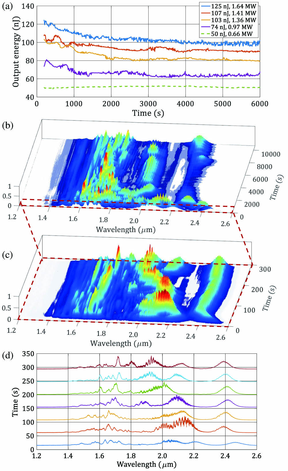
Fig. 1. (a) Time evolution of the output beam power from a 30 cm long GRIN fiber span, for different values of the input peak power. The legend shows the values of input pulse energy and peak power, respectively. (b) Slow temporal evolution of the output spectrum, for fixed input pulse peak power P = 1.41 MW Visualization 1 ). (c) Zoom-in of (b), for the first 285 s. (d) Same spectra of (c) at 7 temporal instants of time.
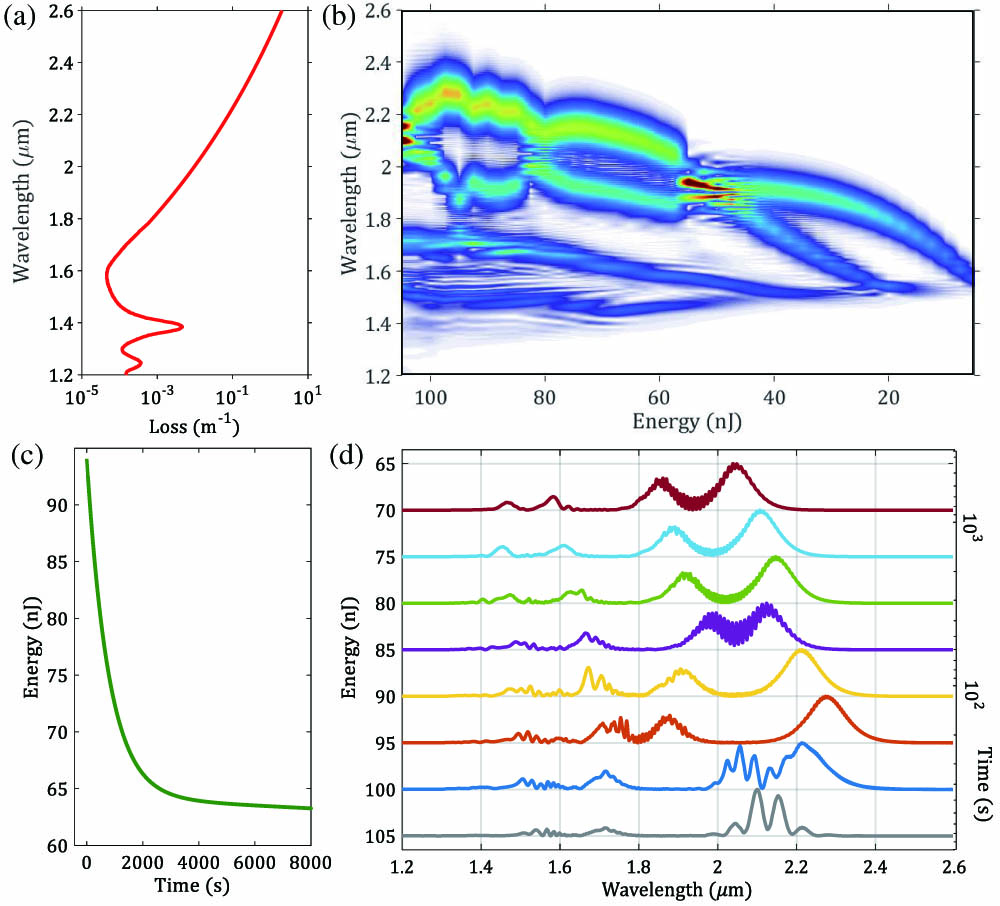
Fig. 2. (a) Wavelength dependence of the linear loss profile in simulations. (b) Numerical simulation of output spectrum changes versus input pulse energy. All parameters are the same as in experiments of Fig. 1 . (c) Relationship between input pulse energy and long time scale obtained by fitting the violet curve in Fig. 1 (a) with an exponential curve. (d) Same spectra of (b) at 8 temporal instants of time.
Fig. 3. Comparison between MPI regime established at 1.03 μm and 1.55 μm of wavelength: (a) transmission; (b), (c) luminescence; (d), (e) damages imaged by optical microscopy. The white bars in (b)–(e) correspond to 100 μm. The input energy and the peak power are E = 323 nJ P = 1.64 MW E = 125 nJ P = 1.64 MW
Fig. 4. X-ray imaging. (a) Radiography of a brand-new GRIN 50/125 fiber. (b) Corresponding intensity profile along the transverse direction x z μ μ x – y
Fig. 5. Analysis of fiber damages. (a) Optical microscope image. (b) Comparison between the intensity profile along the fiber axis in (a) (black curve) with the diameter of the red zone (red area). (c) Variation along z


Set citation alerts for the article
Please enter your email address

© Copyright 2018-2021 | Chinese Laser Press. All Rights Reserved 沪ICP备15018463号-20