
Xu-Sheng Xu, Hao Zhang, Xiang-Yu Kong, Min Wang, Gui-Lu Long, "Frequency-tuning-induced state transfer in optical microcavities," Photonics Res. 8, 490 (2020)
- Photonics Research
- Vol. 8, Issue 4, 490 (2020)
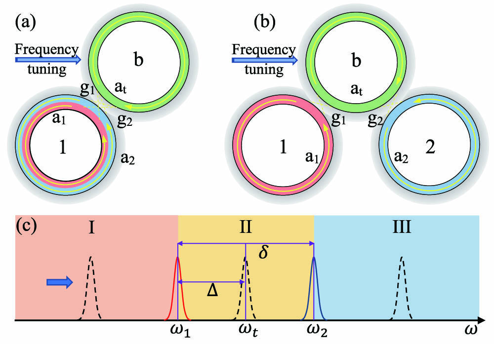
Fig. 1. Schematic diagram for the model of multimode interactions in optical microcavities. All the modes have very narrow linewidths. A mode in one cavity couples to two different optical modes (a) in the same cavity and (b) in two different cavities separately. (c) Resonance frequency tuning of the intermediate cavity to induce state transfer. The tuning domain is divided into three parts labelled I, II, and III.
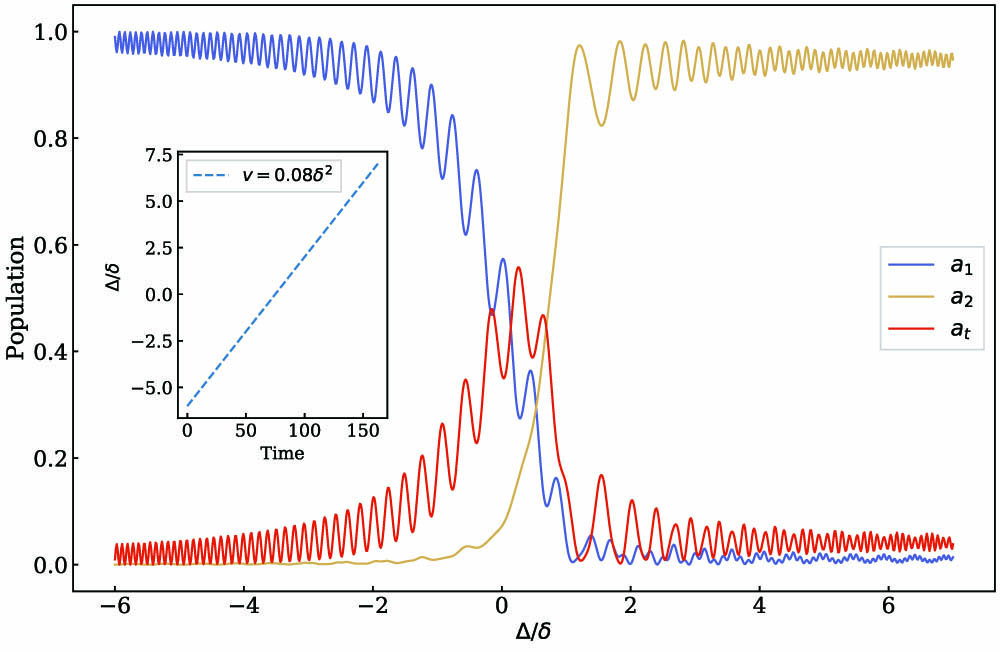
Fig. 2. Result of FIST between a 1 a 2 a t 0.08 δ 2 t δ − 1
Fig. 3. Simulation of final population of mode a 2 d v δ δ 2 P d v = 0.27 δ 2 Δ 0 Δ 0 = ( δ − d ) / 2 P v d = 2.65 δ Δ 0 = − 0.825 δ P d v 10 δ − 1
Fig. 4. Population change with respect to evolution time via sine tuning function. Lines labeled with a 1 a 2 a t
Fig. 5. Simulation of fast FIST from a 1 a 2 3(c) with d = 2.65 δ v = 0.27 δ 2 δ − 1
Fig. 6. Nonreciprocal state transfer between modes a 1 a 2 a 1 a 2 d = 14 δ a 1 a 2 v = 0.1 δ 2 a 2 a 1 log 10 [ P ( a 2 ) ] − log 10 [ P ( a 1 ) ]
Fig. 7. All-optical on-chip microcavity structures. (a) One-dimensional microcavity array. (b) Two-dimensional optical microcavity lattice.


Set citation alerts for the article
Please enter your email address

© Copyright 2018-2021 | Chinese Laser Press. All Rights Reserved 沪ICP备15018463号-20