Microwave technology has been widely used in civilian and defense applications, such as wireless communication, global positioning systems, remote sensing, and satellite surveillance systems ^[1,2]. Nowadays, research on microwave identification techniques is rising, driven by urgent demands for pre-identification of microwave frequencies before taking corresponding countermeasures ^[3,4]. Recently, the emerging topic of photonic-assisted microwave identification has proven a paradigm-shift technique, outperforming traditional electronic solutions in terms of wide frequency coverage and antidisturbance capability. Equally important, the scheme based on photonic integrated chips is of great interest, due to the distinct advances in system miniaturization and low size, weight, and power (SWaP), which is crucial for mobile and airborne applications ^[5–8].

The basic principle of microwave identification is to map the frequency of an unknown microwave signal to a more easily measurable quantity, such as the power or time delay. The schemes using frequency-to-power mapping can implement instantaneous frequency measurement (IFM) of unknown frequencies by constructing an amplitude comparison function (ACF) ^[9]. The ACF with a wider frequency range and a higher gradient was illustrated in a silicon-on-insulator (SOI) microdisk ^[10], a ring resonator ^[11,12], an indium phosphide Mach–Zehnder interferometer (MZI) ^[13], a nonlinear effect chip ^[14], and Bragg gratings ^[15,16]. However, the simultaneous measurement of multiple frequencies is impossible. In addition, various complex forms of microwave signals, such as multiple-frequency (MF) microwaves ^[17–19], chirped-frequency (CF) microwaves ^[20–22], and frequency-hopping (FH) microwaves ^[23,24], are emerging and becoming widely adopted in the real world. For example, the CF and the FH microwave signals are ubiquitous in modern systems, especially in radar systems and communication instruments. The extended frequency band of frequency modulated (FM) signals can enhance network capacity and range resolution due to the larger time-bandwidth product. It is interesting to note that the scheme using frequency-to-time mapping shows the capability of MF measurements in a spectrally cluttered environment and tolerance to the varying input optical power. A tunable Fabry–Perot interferometer used as a scanning receiver with a measurement range of up to 40 GHz and a resolution of 90 MHz was proposed in 1999 ^[25]. Then, various approaches based on frequency-to-time mapping were demonstrated by using a dispersive medium ^[26], a scanning receiver ^[27,28], and a frequency shift loop ^[29]. In 2017, proof-of-concept experiments for both the linearly frequency modulated pulse and frequency Costas coded pulse were demonstrated based on scanning stimulated Brillouin scattering (SBS) ^[30]. However, most of these schemes are based on bulky and discrete components or employing high power. Recently, a milestone demonstration of the MF measurement using a chip-based photonic Brillouin filter was reported, revealing a large measurement range up to 38 GHz and high resolution of less than 1 MHz ^[31]. However, a high optical power of typically more than 100 mW is required to enable nonlinear processing, and the scanning speed is limited by the switching time of the radio frequency (RF) reference signal provide by an expensive and high-frequency microwave generator. In 2018, we demonstrated a photonic multiple microwave frequency measurement system based on a swept frequency silicon microring resonator (MRR) ^[32]. However, the measurement resolution of 5 GHz and the number of measurable frequencies are limited by the small Q-factor. It remains challenging to simultaneously identify different types of microwave frequency signals based on an integrated photonic chip, using ultralow input power and inexpensive components.

In this article, we demonstrate, for the first time, a wideband adaptive microwave frequency identification system (MFIS) using an integrated silicon photonic scanning filter. The system exhibits a versatile capability to identify and quantify single-frequency (SF) signal and complex microwave signals, including MF, CF, and FH microwave signals as well as their combinations. The frequency measurement range is ultrawide, from 1 to 30 GHz, with a high resolution of 375 MHz and a low measurement error of 237.3 MHz. The measurement speed is about 10 ms. This superior performance is enabled by the frequency-to-time mapping using a thermally tunable high Q-factor silicon MRR. This demonstration opens the door for future fully integrated solutions for wideband, adaptive, and high-resolution MFIS.

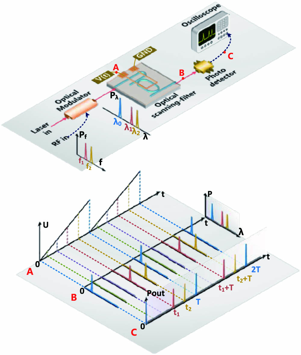
Figure 1 shows the conceptual diagram of the wideband adaptive MFIS. The unknown microwave signal (possibly containing multiple frequencies, i.e., f1 and f2) is modulated onto the optical carrier (with the wavelength of λ0) through the optical intensity modulator (IM) with single sideband modulation. Then, two sidebands of λ1 and λ2 are generated. The key to our approach is the integrated silicon photonic scanning optical filter, with a tunable frequency span of 50 GHz, a narrow bandwidth of ∼300MHz, and an undistorted spectral shape when scanning. The scanning filter is implemented by a thermally tunable high-Q silicon MRR, and the laser wavelength is initially aligned with the resonance of the MRR with no applied voltage. When driven by a periodic sawtooth voltage, the resonant wavelength of the MRR will experience a periodic redshift, exhibiting a periodic scanning filter. When the scanning filter matches the measured sidebands (λ1 or λ2), a temporal pulse will appear at the corresponding time (t1 or t2). After being detected by a low-speed photodetector and recorded by a low-speed oscilloscope, the unknown microwave frequencies will be mapped to the temporal pulses in sequence. The driving voltage for the MRR is a periodic sawtooth function, and the resonance drift is proportional to the power of the driving signals; thus, the resonance drift varies quadratically with the voltage and time variables. Therefore, the frequency-to-time mapping function of the unknown signal can be expressed as where funknown is the unknown frequency of the microwave signal, t denotes the time variable, and A, B, and C are constants determined by the practical system, which should be calibrated in advance. In practice, the laser wavelength should be a little mismatched with the resonant wavelength of the microring for around 0.5 GHz in the initial state, so that the microring could operate stably without thermal instability. Besides, there is a discontinuous point between two periods of sawtooth signals. This means that the scanning filter has scanned all the sidebands at the discontinuous point. Thus, a sharp pulse is formed. This sharp pulse is helpful to define the baseline and synchronize the input sawtooth signal and the output intensity waveform.

The experimental configuration for the wideband adaptive microwave frequency identification system is presented in Fig. 2. The optical carrier is provided by a tunable laser source (TLS, Alnair Labs TLG-200) with a power of 10 dBm. After a polarization controller, the unknown radio frequency signal is modulated to the optical carrier by an intensity modulator. The unknown RF signals of different types are generated by an RF arbitrary-waveform generator (Keysight M8195A). The bias voltage of the IM is set as 3.1 V to ensure proper carrier suppression. The operating RF amplitude range of the IM is about 300 mV to 3 V, and the RF signal in this range can be measured theoretically. Limited by the output amplitude of the arbitrary waveform generator (AWG), we verified that 20 GHz RF signals ranging from 300 mV to 1 V can be identified. The optical filter is used to suppress the lower sideband to achieve an optical single-sideband modulated signal (OSSB). The optical filter is a ramp filter, and its loss decreases with increasing wavelength. Therefore, the power of the lower sideband decreases with the increasing of modulation frequency. Then, the generated OSSB is amplified by an erbium-doped fiber amplifier (EDFA) to compensate the link loss and is injected into the chip after a polarization controller (PC2). The thermal electrode of the MRR is controlled by an electrical arbitrary waveform generator (EAWG, Agilent 33250A). By loading a periodic sawtooth voltage to the MRR, the resonance wavelength will experience a periodic redshift; thus, a periodic scanning filter can be formed. The second EDFA (EDFA2) is employed to compensate the chip loss, and the attenuator is used to protect the low-speed photodetector (PD, KG-PR-200M-A-FC). Finally, the unknown microwave frequencies will be mapped to the time domain and recorded as a series of pulse signals by an oscilloscope (Agilent dso7054A).

The chip-based scanning filter is implemented with a high-Q silicon MRR chip. The chip was fabricated on a standard SOI wafer at IME using a complementary metal-oxide-semiconductor compatible technique. Figure 3(a) shows a micrograph of the high-Q MRR, which consists of a race-track ring resonator, two straight waveguides, and a pair of thermal electrodes. The radius of the half-ring is set to 20 μm to reduce the footprint. The widths of the half-rings and the straight waveguides are set to 500 nm to guarantee fundamental mode transmission. The width of the race-track region is set to 2 μm to decrease the scattering loss. To convert the TE mode from the fundamental mode waveguide to the multimode waveguide, a linear adiabatic taper with a length of 40 μm is used. A detailed description of the MRR fabrication can be found in Ref. ^[33].

To quantify the relationship between the spectrum drift and the applied voltage, the spectral response of the MRR at different direct current (DC) voltages is measured with an optical spectrum analyzer (OSA) [shown in Fig. 3(b)] with a free spectral range of 50 GHz. The resolution of the OSA is only 0.02 nm, so we use the method in Ref. ^[34] to characterize the Q-factor of the MRR. According to accurate measurements made with a vector network analyzer, we finally confirm that the 3 dB bandwidth of the MRR is 325 MHz at the wavelength of 1550.12 nm, implying a Q-factor of ∼600,000. The measured wavelength drift has a quadratic function relationship with the loaded voltage as we expected, as shown in Fig. 3(c). When the applied voltage is 3.4 V, the wavelength drift is 0.264 nm, which is equivalent to 33 GHz. In the experiment, a periodic sawtooth voltage is applied on the MRR, ranging from 0 to 3.3 V with a period of 10 ms. The response rate of the MRR heater is approximately 14 kHz ^[35]. Due to the high loss of the RF cable and IM above 30 GHz, the effective measurement bandwidth is limited from 1 to 30 GHz. Then, we scan the given microwave frequency from 1 to 30 GHz and record the emerging time of temporal pulses. The input RF amplitude is set at 500 mV for all the test signals. As a result, the functional relationship between the microwave frequency and the pulse delay is determined as shown in Fig. 3(d), which is the lookup table for estimating the unknown frequency. Based on the MFIS, we first verify the measurement for a time-invariant SF signal, a microwave signal that has a single frequency and does not change over time. Then, we collect 221 measured samples for different time-invariant single frequencies to evaluate system performance. In Fig. 3(e), the red dots and blue dots show the frequency estimated through the MFIS and the measured error for each of the test tones, and the measurement error histogram shows the distribution of different errors. The root-mean-square error can be calculated by σRF=∑i=1N[fe(i)−fin(i)]2N.(2)Here, σRF is the root-mean-square error, fin is the input frequency, fe is the measured frequency, and N is the measurement number. Figure 3(e) indicates that the system has the ability to measure broadband microwave frequencies from 1 to 30 GHz with a root-mean-square error of ∼237.3MHz. The measurement error comes mainly from two aspects. First, the scanning filter is not an ideal narrowband filter in the real world, which means that the measurement accuracy will be limited by the 3 dB bandwidth of the filter. Therefore, the measurement accuracy can be further improved by using an ultrahigh-Q filter. In addition, the increased measurement error at high frequencies observed in Fig. 3(e) is attributed to the higher loss of high-frequency microwave signals caused by the RF cable and IM.

The method of frequency-to-time mapping is a powerful tool for time-invariant MF identification and measurement. To verify the capability of MF measurement, we prepared several samples to be measured of time-invariant MF microwave signals with an RF arbitrary waveform generator. Finally, the multiple emerging pulses on the oscilloscope represent the corresponding input frequencies, as shown in Fig. 4. First, the MF signal contains a random combination of 2, 10, and 12 GHz as the prepared sample, and the measured values in our system are 1.83, 10, and 12.02 GHz, respectively [see Fig. 4(a)]. Then, we prepared a complex sample of MF signals, ranging from 2 to 30 GHz, stepped by 2 GHz. It can be seen that the 15 measured frequencies are evenly spaced in the temporal waveform [see Fig. 4(b)]. One may note that temporal pulses exceeding 20 GHz have a distinct attenuation. Thus, we measured the RF response of the IM by a vector network analyzer (VNA, Anritsu MS4647B) from 0 to 40 GHz, as shown in Fig. 5. As we can see, the transmission decreases with the increased frequency, and the transmission loss is particularly high exceeding 20 GHz. This is mainly caused by the high loss of the IM and RF cable at high frequency. The high loss will make it difficult to detect high-frequency signals, so we use a ramp filter to compensate the frequency loss. However, due to the double loss slope, the detected power above 20 GHz is still small. Furthermore, if the frequency-dependent loss of the link is accurately estimated, it can be calibrated in post-processing.

To verify the frequency resolution for multiple tones, we prepared a microwave sample containing closely spaced frequencies ranging from 2 to 20 GHz, stepped by 0.5 GHz. As we can see from Fig. 4(c), 37 intensive frequencies can be accurately distinguished and measured in the waveform. In the end, to estimate the frequency resolution, a two-tone frequency signal of 2 and 2.375 GHz was injected into the MFIS, and the measured values are 1.887 and 2.203 GHz, respectively [see Fig. 4(d)]. For all the above signals, the measured deviation is less than 300 MHz for each tone. We define the frequency resolution as the gap between two adjacent pulses when the power of the intersection is at half the maximum power. From the measured result for the two tones at 2 and 2.375 GHz, we can see that the two tones are just distinguishable and that the frequency resolution is 375 MHz. Because the 3 dB bandwidth of the MRR is approximately 325 MHz at a wavelength of 1550 nm, the frequency resolution is slightly larger than 325 MHz, taking the link degradation into consideration. To summarize, we have successfully demonstrated the capabilities of time-invariant MF identification in terms of frequency range (2–30 GHz), frequency quantity (as many as 37 frequencies), and frequency resolution (∼375MHz).

The identification for FM signals is based on statistic measurement. Here, we will present the detailed theoretical model and simulations. In one scanning period, the scanning frequency of the filter exhibits a quadratic function relationship with the time as shown in Fig. 6(a), and we define this frequency as fs(t). At the same time, the chirped frequency and hopping frequency as functions of time are shown in Figs. 6(b) and 6(c). We define the input instantaneous frequency of the chirped frequency and hopping frequency as fin(t). Thus, there is a difference between the scanning frequency and the input frequency at a certain moment. The frequency deviation can be defined as fd(t)=fs(t)−fin(t).(3)When the input instantaneous frequency is close to the scanning frequency, the detected optical power is high. The equation is obtained by theoretical approximation. The relationship between the output power and the frequency deviation yields to the filter distribution. In the simulations, we use a Gaussian function to approximate the filter shape. Therefore, a Gaussian function is used to describe the output power with respect to the frequency deviation as Pout(t)=e−[fd(t)k]2,(4)where k is a constant, related to the filter bandwidth. The measured frequency resolution is 375 MHz for the scanning filter. This means when fd(t) equals 375 MHz, the output power is 0.5. Then, we can deduce that k=450.4MHz. In the end, the detected temporal waveforms can be calculated based on Eq. (4) according to time-to-frequency mapping.

Figure 7 shows simulated results for FM microwave signals with different frequency spans and center frequencies. In Figs. 7(a) and 7(b), the two CF samples are chosen by different spans of 16 and 1 GHz at the same center frequency of 20 GHz. In Figs. 7(c) and 7(d), the two FH samples are chosen from 2 to 18 GHz stepped by 16 and 0.5 GHz. As we can see, the FM microwave signals can be identified from the simulated results. In addition, the measured results are consistent with the simulated results according to the next section. The imbalance of the measured amplitude is caused by the radio frequency loss of the IM response at high frequency.

CF microwave pulses have many important applications in modern radar and wireless communication. In these situations, it is still a challenge to estimate the frequency band of a CF microwave pulse before taking corresponding countermeasures. Fortunately, the proposed MFIS is capable of identifying a CF microwave pulse due to the approach of frequency-to-time mapping. In the experiment, CF microwave pulses with different central frequencies and frequency spans are generated by the RF AWG. The pulse width and repeat interval are set to 1.6 and 4 μs, respectively. Because the period of the scanning filter is 10 ms, the MFIS performs a statistical measurement of 2500 pulses during a period of 10 ms. At a random time within the period, the recorded power is related to the deviation between the instantaneous input frequency and the instantaneous scanning frequency. Thus, the measured waveform is an intensity envelope with random power values filled, as shown in Fig. 8. The measured frequency band is defined as the full width at half-maximum (FWHM) normalized amplitude. Figures 8(a)–8(c) show the measurement comparison between a commercial electrical spectrum analyzer (ESA, red line) and our MFIS (blue line), where the CF microwave pulses have different frequency spans of 16, 4, and 1 GHz but the same central frequency of 20 GHz. In addition, Figs. 8(e)–8(g) show the measurement comparison between the commercial ESA and our MFIS for CF microwave pulses with the same frequency span (4 GHz) but increased central frequencies of 4, 16, and 24 GHz. For a more intuitive display, Figs. 8(d) and 8(h) exhibit the measured and real frequency bars for different samples of CF microwave signals. It can be seen that the measured frequency span well matches the input frequency span. To quantitatively analyze the measurement results, the parameters of bandwidth error and central frequency error are defined as σband=∑i=1N[Be(i)−Bin(i)Bin(i)]2N,(5)σcenter=∑i=1N[Ce(i)−Cin(i)]2N.(6)Here, σband is the root-mean-square error of the measured relative bandwidth, and Be(i) and Bin(i) are the measured and real bandwidths for the ith sample, respectively. σcenter is the root-mean-square error of the measured central frequency, and Ce(i) and Cin(i) are the measured and real central frequencies, respectively. After the calculation, σband and σcenter for the central frequency invariant microwave signals in Fig. 8(d) are 6.54% and 499.7 MHz, respectively. σband and σcenter for the frequency band invariant microwave signals in Fig. 8(h) are 7.35% and 178.6 MHz, respectively. Despite the small measurement error caused by the instability of the filter, our MFIS shows the ability to identify the frequency band of CF microwave pulses in a simple manner.

Similar to the CF microwave signal, the FH microwave signal is a type of time-varying signal, and the corresponding measurement is based on a statistical method as well. First, the FH microwave signals are prepared with a frequency span of 2 to 18 GHz, hopped by a series of steps. The duration per tone is set to 500 ns. The FH microwave signals stepped by 16, 4, 1, and 0.5 GHz are measured by both the MFIS (blue line) and the ESA (red line), and the measured results are shown in Fig. 9. When there are only two frequencies of 2 and 18 GHz, we achieve two pulse envelopes with random amplitude filled. When the step number of FH signals is increased, we measure more pulse envelopes in the MFIS, which are well aligned with the real frequency measured in the ESA. The measured error for FH microwave signals is approximately 166.3 MHz.

From the experiments reported in Figs. 8 and 9, we can see that the measurement results are comparable with a commercial ESA and proved to be accurate. Different from a commercial ESA, the applications of the proposed scheme are to identify different complex microwave signals and extract frequency information. Besides, the proposed scheme has potential for high-frequency and wideband microwave frequency identification. In addition, the photonics-based scheme has a low SWaP for further mobile and avionic applications.

As described in the above demonstrations, we have implemented the measurement of four types of typical microwave signals. Obviously, the measured waveforms of these four types have distinguishable characteristics, which are summarized in Table 1. For the FM signals, the output waveform is the statistics of output power, which is related to the frequency deviation. In one scanning period, the frequency deviation for FM signals varies discontinuously. In contrast, the frequency deviation changes continuously for the time-invariant microwave frequency. Therefore, if the measured pulse is filled with random power, we can judge that it is an FM signal based on a statistical measurement. The simulated results in Fig. 7 have proven it. Although FH and CF microwave signals are based on statistical measurements, we can further distinguish them by judging whether the pulse envelope is continuous or discrete. In addition, if the measured pulse is hollow without being filled with random powers, we can judge that it is a time-invariant signal. By counting the number of pulses, we can check whether the signal is SF or MF.

Our system has the ability to identify more complex microwave signals, even when various microwave formations exist simultaneously, such as a combination of multitype microwave signals. To verify this powerful function, we demonstrate frequency identification experiments for different combinations of two-type microwave signals, as shown in Fig. 10. First, simultaneous FH signals and CF signals are generated and combined using the RF AWG. The parameters are divided into four groups: FH (2–6 GHz, stepped by 2 GHz) and CF (8–12 GHz); FH (2–6 GHz, stepped by 1 GHz) and CF (8–12 GHz); FH (8–12 GHz, stepped by 1 GHz) and CF (2–6 GHz); and FH (8–12 GHz, stepped by 2 GHz) and CF (2–6 GHz). As shown in Fig. 10(a), the measured pulses are filled with random power, with continuous and discrete pulse envelopes both appearing in the result. According to the previous criteria, we can judge that the test signals contain both FH and CF signals, and the frequency values can be read out readily. Next, simultaneous SF signals and CF signals are generated and combined using the RF AWG, as shown in Fig. 10(b). These signals can overlap in the frequency domain and are divided into four groups as well: SF (6 GHz) and CF (8–12 GHz); SF (12 GHz) and CF (8–12 GHz); SF (20 GHz) and CF (6–14 GHz); and SF (10 GHz) and CF (6–14 GHz). When there is no overlap between the SF and CF signals, the results are composed of a hollow pulse and a filled continuous pulse. When SF and CF signals have overlap regions in the frequency domain, the measured waveforms have overlap as well. However, it is worth noting that the power of the overlap region is doubled, and the hollow appears at the bottom of the waveform. According to these characteristics, the combination of an SF and a CF can also be precisely identified and measured. Last, simultaneous SF signals and FH signals are generated and combined using the RF AWG, as shown in Fig. 10(c). The FH signal is prepared from 4 to 12 GHz stepped by 2 GHz. When the SF signal is 20 GHz, the measured waveform is clearly composed of a hollow pulse and filled discrete pulses. When the SF signal is with the same frequency (12 GHz) as the FH signal, the corresponding measured power is doubled and hollow at the bottom. When the SF signal is located in the interval of the FH frequencies (i.e., 11 GHz or 5 GHz), the measured waveforms still clearly contain a hollow pulse and filled discrete pulses. For the above results, the σband and σcenter for CF signals are 5.48% and 256.2 MHz, and the σRF for FH and SF signals is 154.1 MHz. Therefore, our MFIS has demonstrated the powerful capability of identifying simultaneous linear combinations of multitype microwave signals with high resolution.

In the above experiment, we have demonstrated a powerful and wideband adaptive MFIS. Our MFIS has successfully identified SF signals and complex microwave signals, including MF, CF, and FH microwave signals and their combinations. Moreover, the frequency components of the signal can be measured in an accurate manner. In fact, our MFIS also has the ability to measure the relative amplitudes of unknown microwave signals. For example, an SF signal at 20 GHz is measured by our MFIS, and a temporal pulse is observed at the measured time based on frequency-to-time mapping. Because the pulse amplitude is positively correlated to the input microwave power, we can estimate the microwave power by measuring the pulse amplitude. Then, we change the input microwave amplitude from 0.3 to 1 V, and the corresponding measured pulse amplitude is recorded from the oscilloscope. Figure 11 shows the measured amplitude as a function of input microwave amplitude. The monotony of the curve manifests the possibility of measuring the power of each frequency within a complex microwave circumstance. One may note that the input–output amplitude relationship does not vary linearly, which is caused by the nonlinear modulation of the IM. In real applications of amplitude measurements, the modulator bandwidth, modulator linearity, and acceptable power range of microwave signals should all be taken into consideration.

In all the experiments, the input RF amplitude spans from 300 mV to 1 V. However, in the real-world applications, the received RF signal is always at a low power level. The dynamic range of the system is mainly limited by the IM, which is used to convert the microwave frequency to the optical domain. Thus, the RF input power should be able to drive the IM. There are two possible methods for improving the RF link performance. One is expanding the dynamic range of the IM, and the other is to add an RF amplifier before the RF input.

We compare the performance of existing MFISs, as shown in Table 2. The proposed scheme uses an integrated photonic filter to form a linear system and avoids high optical power for operation. Compared with our previous work, the key parameters of measurement range and accuracy are greatly improved. Additionally, our design is an important step forward by demonstrating its capabilities to identify a number of different complex microwave signals, which can extend the applications. Meanwhile, the demonstrated device does not offer the capability of IFM limited by the scanning time (10 ms). Therefore, the applications of the proposed MFIS are focused on frequency-type recognition and statistical quantitative analysis.

Finally, if one can monolithically integrate all components of the wideband adaptive MFIS, the photonic MFIS can move toward a more practical path. Recently, reports about room-temperature lasers grown on silicon ^[36,37] and high-speed silicon modulators ^[38,39] give us confidence in the possibility of a monolithically integrated MFIS. In particular, a crucial advantage of our scheme is that the measurement device uses a low-speed PD, which can greatly reduce the design difficulty of the whole chip. In brief, the proposed integrated silicon photonic scanning filter suggests an attractive potential for a chip-scale microwave photonic system.

In conclusion, we have proposed a simple method for wideband adaptive microwave frequency identification using an integrated silicon photonic scanning filter. Four types of typical microwave signals, namely, SF, MF, CF, and FH microwave signals, and even their combinations, can be classified according to the features of the measured waveforms. The frequency identification range is from 1 to 30 GHz, with a resolution of 375 MHz and a low measurement error of 237.3 MHz. In consideration of the breakthrough of laser diodes, high-speed modulators, PD, and scanning filters based on SOI platforms, our method will pave the way for monolithically integrated MFIS chips with a compact size, low cost, and spectrally cluttered scenario.

Acknowledgment. We thank Prof. Jianping Yao from the University of Ottawa for his fruitful discussion and suggestions.

References

[1] K. Chang. RF and Microwave Wireless Systems(2004).
[2] F. Neri. Introduction to Electronic Defense Systems(2006).
[3] J. R. Tuttle. Traditional and emerging technologies and applications in the radio frequency identification (RFID) industry. IEEE Radio Frequency Integrated Circuits (RFIC) Symposium, 5-8(1997).
[16] M. Burla, X. Wang, M. Li, L. Chrostowski, J. Azaña. On-chip instantaneous microwave frequency measurement system based on a waveguide Bragg grating on silicon. CLEO 2015, STh4F.7(2015).
[18] D. B. Hunter, L. G. Edvell, M. A. Englund. Wideband microwave photonic channelised receiver. International Topical Meeting on Microwave Photonics, 249-252(2005).
[21] W. Zhang, J. Zhang, J. Yao. Largely chirped microwave waveform generation using a silicon-based on-chip optical spectral shaper. Microwave Photonics (MWP) and International Topical Meeting on 9th Asia-Pacific Microwave Photonics Conference (APMP), 51-53(2014).
[23] J. Yao, W. Li, W. Zhang. Frequency-hopping microwave waveform generation based on a frequency-tunable optoelectronic oscillator. Optical Fiber Communication Conference, W1J.2(2014).
[38] Z. Pan, X. Xu, C.-J. Chung, H. Dalir, H. Yan, K. Chen, Y. Wang, R. T. Chen. High speed modulator based on electro-optic polymer infiltrated subwavelength grating waveguide ring resonator. Optical Fiber Communication Conference, M2I.2(2018).
[39] J. Sun, M. Sakib, J. Driscoll, R. Kumar, H. Jayatilleka, Y. Chetrit, H. Rong. A 128 Gb/s PAM4 silicon microring modulator. Optical Fiber Communication Conference, Th4A.7(2018).