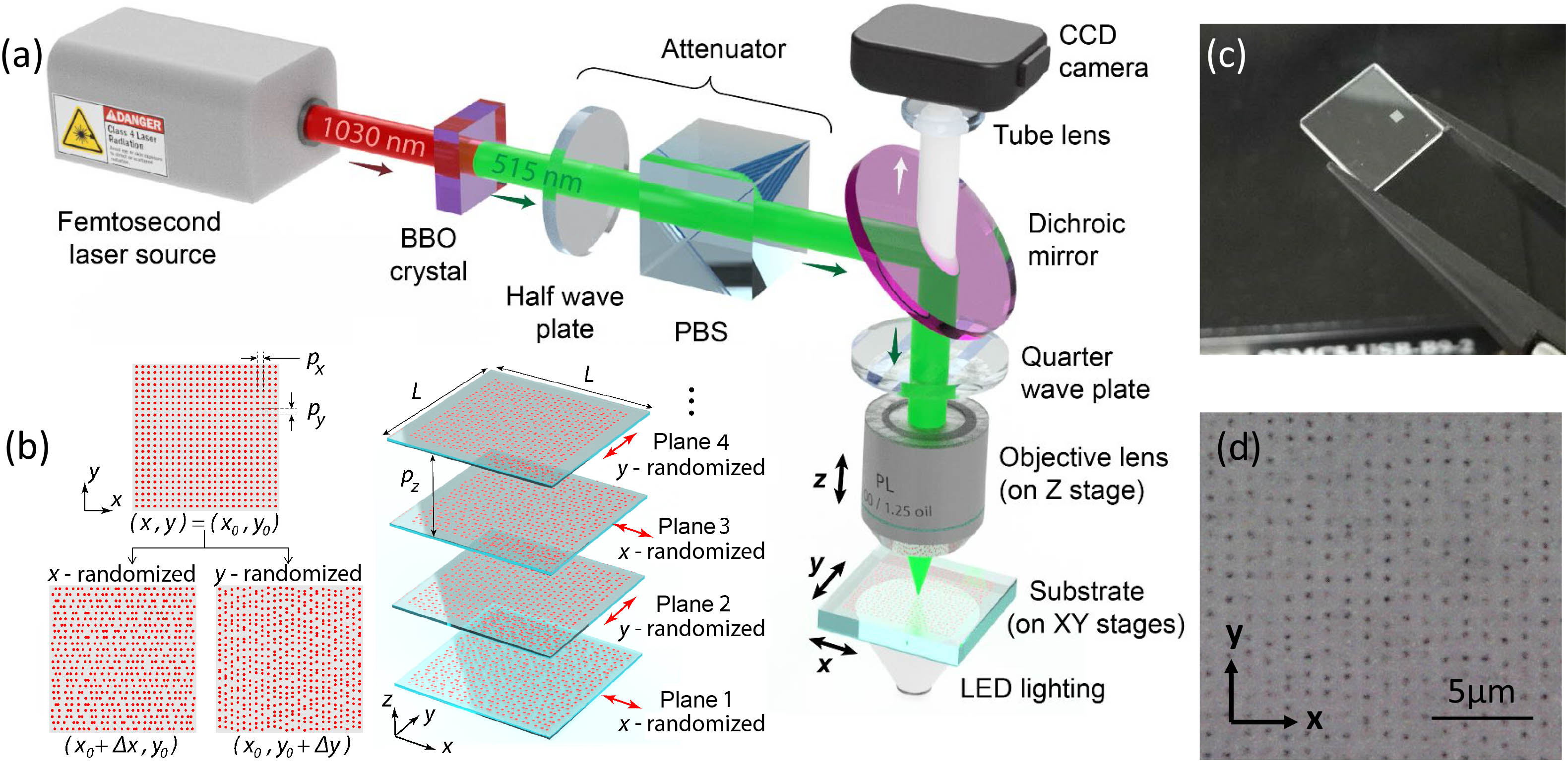
Fig. 1. Production of pseudo-random scattering chips. (a) Femtosecond laser writing experimental setup for scattering medium. (b) Design of scattering planes: a regular grid of scattering voids (red dots) is randomized in either the x or y direction, by adding uniformly distributed random offsets (±0.4  μm) to either the x or y coordinates for alternating planes. Mean transverse pitch px=py=1  μm; plane spacing pz=5  μm. (c) Photograph of 10  mm×10  mm×1  mm silica substrate and 1  mm×1  mm scattering pattern. (d) Microscope image of one plane of a y-axis randomized scattering pattern.

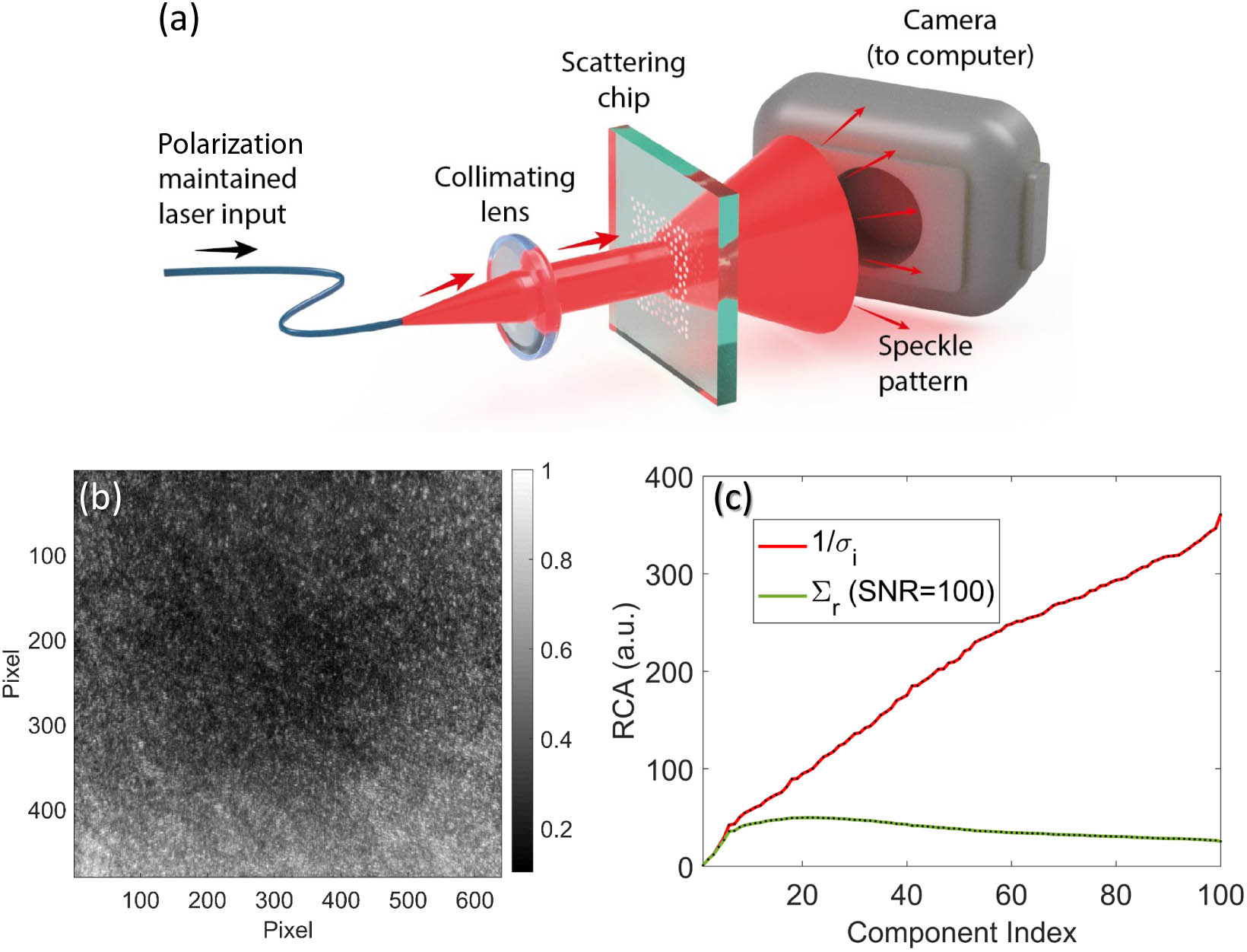
Fig. 2. (a) Scattering spectrometer setup. (b) Example of speckle intensity pattern captured with camera. (c) Inverse of normalized singular values before (red) and after (green) applying Wiener filter. The signal-to-noise ratio (SNR) of the system is set to 100. RCA is the reciprocal component amplitude.

Fig. 3. Cropping and binning effect on speckle stability. (a) Unmodified speckle time-wise displacement in x and y. Note: for clarity, only first 24 h of displacement is plotted. The behavior of a fluctuation of x and y coordinates remained the same at all time. (b) Speckle temporal stability (RMS difference) for unmodified, binned, and cropped speckle patterns. Note: dashed flat line indicates period when laser was turned off. (c) Example speckle patterns with and without cropping and binning. Pixel peak intensity value is normalized to unity.

Fig. 4. Wavelength reconstruction stability test for (a) long-term fixed wavelength over 168 h (chip), (b) long-term fixed wavelength over 12 h (50 cm MMF), and (c) short-term wavelength steps over a total of 180 h, comparing the reconstructed and OSA-measured reference wavelengths (chip).

Fig. 5. (a) Reconstruction of a spectrum with two wavelengths separated by 0.1 nm. (b) Spectrum with sinusoidal shape (black), its ideal reconstruction from the calibration data (red), and its reconstruction from test speckle patterns (blue). (c) Impact of binning on reconstructed spectrum, showing an increase in standard deviation. (d) Impact of binning on reconstructed spectrum, showing reduction in spectral contrast. ϵstd is the standard error of the obtained spectra.

Fig. 6. Impact of cropping and binning on spectral reconstruction. Spectrum matrices for (a) full image size, (b) nbin=5, and (c) nbin=20. (d) Standard reconstruction error versus binning order nbin. (e) Spectrum matrices for ncrop=5 and (f) ncrop=20. (g) Standard reconstruction error versus cropping order ncrop; red bars indicate range of standard errors for different positions of cropping window over the main diagonal. Blue line indicates average from all cropping area positions for given order. Spectrum matrices in (a)–(f) are normalized to unity; better contrast on the diagonal line signal means better correlation between test and calibration wavelength.