Ultra-short pulse fiber amplifier model based on recurrent neural network (Invited)

Yiwen Zhang; Yu Cai; Lixin Yuan; Minglie Hu

doi:10.3788/IRLA20210857

Journals >Infrared and Laser Engineering >Volume 51 >Issue 1 >Page 20210857 > Article

Infrared and Laser Engineering
Vol. 51, Issue 1, 20210857 (2022)

Ultra-short pulse fiber amplifier model based on recurrent neural network (Invited)

Yiwen Zhang, Yu Cai, Lixin Yuan, and Minglie Hu

Author Affiliations

Ultrafast Laser Laboratory, College of Precision Instruments and Opto-Electronics Engineering, Tianjin University, Tianjin 300072, China

show less

DOI: 10.3788/IRLA20210857 Cite this Article

Yiwen Zhang, Yu Cai, Lixin Yuan, Minglie Hu. Ultra-short pulse fiber amplifier model based on recurrent neural network (Invited)[J]. Infrared and Laser Engineering, 2022, 51(1): 20210857 Copy Citation Text

show less

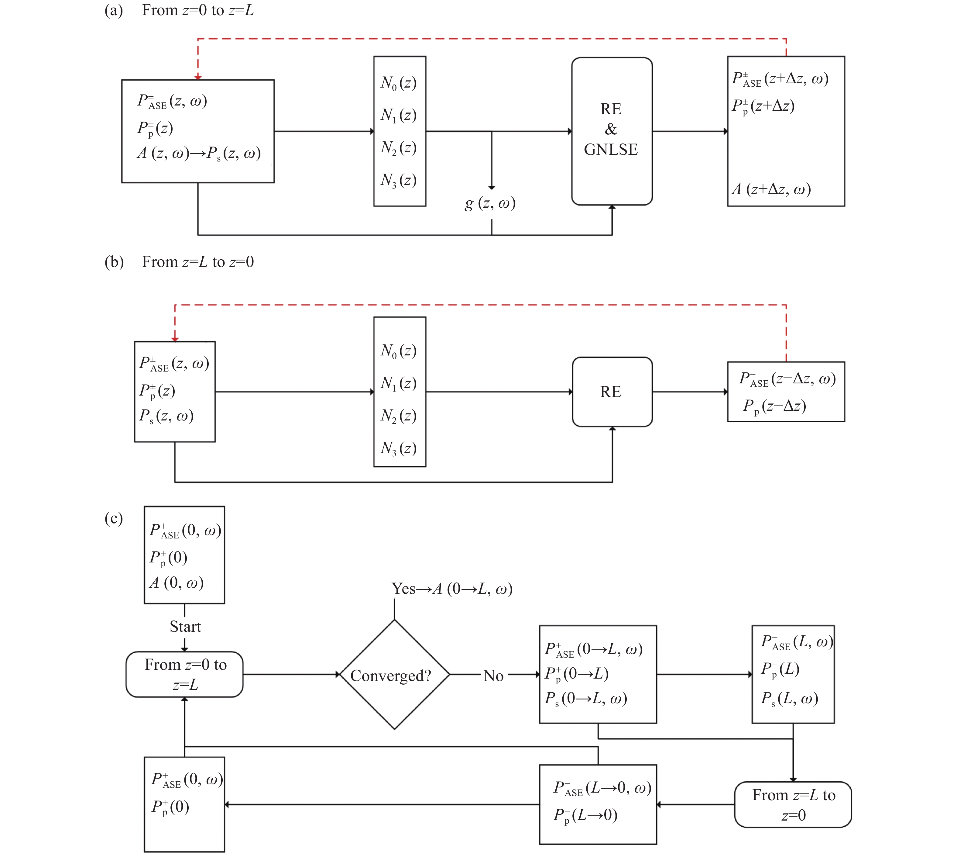
Fig. 1. Schematic of numerical calculationsmodel of fiber amplifiers

Download full size | View in the Article

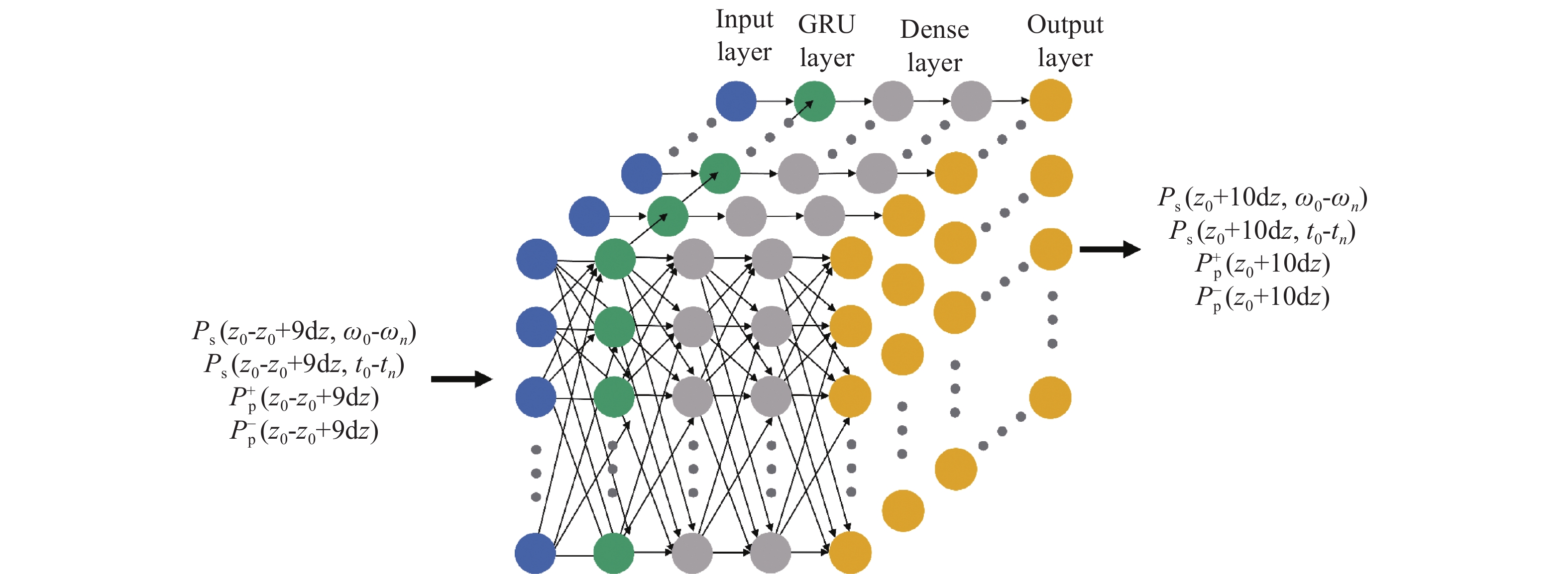
Fig. 2. Schematic of the recurrent neural network architecture

Download full size | View in the Article

Fig. 3. Evolution of pulses calculated using NLSE&RE and RNN respectively. (a) Time domain evolution; (b) Frequency domain evolution; (c) Pulse width (blue line) and spectral width (red line)

Download full size | View in the Article

Fig. 4. Time domain and frequency of pulses at different transmission distances calculated using NLSE&RE (red dotted line) and RNN (blue solid line) respectively

Download full size | View in the Article

Fig. 5. Calculation time versus number of grid points and calculation steps by using NLSE&RE and RNN respectively

Download full size | View in the Article

Fig. 6. Comparison of experimental results with simulation results. (a) Amplifier power; (b) Time domain of output pulses; (c) Spectrum of output pulses, where GNLSE&RE calculated results are red dotted lines, RNN predicted results are blue solid lines and experimental results are black solid lines

Download full size | View in the Article

Parameters	Value	Source	Parameters	Value	Source
${\lambda _0}/ {{\text{nm}}} $	1 975	Measured	${\lambda _{\text{p}}}/ {{\text{nm}}} $	793	Measured
${\sigma _{\text{a} } } \left({ {\lambda _j} } \right)/ { { {\text{m} }^{\text{2} } } }$	Fitted	Jackson[16]	${\sigma _{\text{a} } } \left( { {\lambda _{\text{p} } } } \right)/ { { {\text{m} }^{\text{2} } } }$	$6 \times {10^{ - 25}}$	Smith[20]
${\sigma _{\text{e} } } \left({ {\lambda _j} } \right)/ { { {\text{m} }^{\text{2} } } }$	Fitted	Jackson[16]	${\sigma _{\text{e} } }\left( { {\lambda _{\text{p} } } } \right)/ { { {\text{m} }^{\text{2} } } }$	$5 \times {10^{ - 26}}$	Smith[20]
${N_{\text{d}}}/ {{{\text{m}}^{-3}}} $	$1.7 \times {10^{26}}$	NUFERN	$V$	3.02	NUFERN
${D_{ {\text{core} } } }/ { {\text{μ} }{\rm{m} } }$	10	NUFERN	${D_{ {\text{clad} } } }/ { {\text{μ } } }{\rm{m} }$	130	NUFERN
${A_{\rm{eff} } }/{ {\text{μ } }{ {\rm{m} }^{\text{2} } } }$	72.7	Calculated[21]	${A_{\text{p} } }/ {\text{μ } } {\text{m} }^{\text{2} }$	$1.40 \times {10^4}$	Calculated[21]
$ {\varGamma _{\text{s}}} $	0.88	Calculated[21]	$ {\varGamma _{\text{p}}} $	$5.6 \times {10^{ - 3}}$	Calculated[21]
${A_{30}}/ {{{\text{s}}^{{{ - 1}}}}} $	0		${A_{31}}/ {{{\text{s}}^{{{ - 1}}}}} $	$7 \times {10^4}$	Jackson[16]
${A_{32}}/ {{{\text{s}}^{{{ - 1}}}}} $	0		${A_{20}}/ {{{\text{s}}^{{{ - 1}}}}} $	0
${A_{21}}/ {{{\text{s}}^{{{ - 1}}}}} $	0		${A_{10}}/ {{{\text{s}}^{{{ - 1}}}}} $	3000	Jackson[16]
${k_{3011} }/ { { {\text{m} }^{\text{3} } } \cdot { {\text{s} }^{ { { - 1} } } } }$	$2 \times {10^{ - 22}}$	Smith[20]	$ {k_{1130}}/ {{{\text{m}}^{\text{3}}} \cdot {{\text{s}}^{{{ - 1}}}}} $	$2 \times {10^{ - 23}}$	Smith[20]
${k_{2011} }/ { { {\text{m} }^{\text{3} } } \cdot { {\text{s} }^{ { { - 1} } } } } $	0		$ {k_{1120}}/ {{{\text{m}}^{\text{3}}} \cdot {{\text{s}}^{{{ - 1}}}}} $	0
${\alpha _{\text{s} } }/ { { {\text{m} }^{ { { - 1} } } }}$	$2.3 \times {10^{ - 3}}$	Jackson[16]	${\alpha _{_{\text{p} } } } / { { {\text{m} }^{ { { - 1} } } }}$	$1.2 \times {10^{ - 2}}$	Jackson[16]
${\beta _2}/ { {\text{p} }{ {\text{s} }^{\text{2} } }\cdot{\text{k} }{ {\text{m} }^{ { { - 1} } } } }$	−88	NUFERN	${\beta _3}/ { {\text{p} }{ {\text{s} }^{\text{3} } }\cdot{\text{k} }{ {\text{m} }^{ { { - 1} } } }}$	+0.28	NUFERN
${n_2}/ { { {\text{m} }^{\text{2} } }\cdot{ {\text{W} }^{ { { - 1} } } } }$	$2.3 \times {10^{ - 20}}$	Agrawal[18]	$\gamma / { { {\text{m} }^{ - 1} }\cdot{ {\text{W} }^{ { { - 1} } } }}$	0.0010	Calculated[18]

Table 1. Parameters used in the simulation

Yiwen Zhang, Yu Cai, Lixin Yuan, Minglie Hu. Ultra-short pulse fiber amplifier model based on recurrent neural network (Invited)[J]. Infrared and Laser Engineering, 2022, 51(1): 20210857

Download Citation

Tools

Save the article for my favorites

Paper Information