• Advanced Photonics
  • Vol. 1, Issue 6, 066001 (2019)
Jian Zhao1、†,*, Yangyang Sun1, Hongbo Zhu2, Zheyuan Zhu1, Jose E. Antonio-Lopez1, Rodrigo Amezcua Correa1, Shuo Pang1, and Axel Schulzgen1
Author Affiliations
  • 1University of Central Florida, CREOL, The College of Optics and Photonics, Orlando, Florida, United States
  • 2Chinese Academy of Sciences, Changchun Institute of Optics, Fine Mechanics and Physics, State Key Laboratory of Luminescence and Applications, Changchun, China
  • show less
    DOI: 10.1117/1.AP.1.6.066001 Cite this Article Set citation alerts
    Jian Zhao, Yangyang Sun, Hongbo Zhu, Zheyuan Zhu, Jose E. Antonio-Lopez, Rodrigo Amezcua Correa, Shuo Pang, Axel Schulzgen. Deep-learning cell imaging through Anderson localizing optical fiber[J]. Advanced Photonics, 2019, 1(6): 066001 Copy Citation Text show less
    Schematic of the cell imaging setup and the architecture of the DCNN.
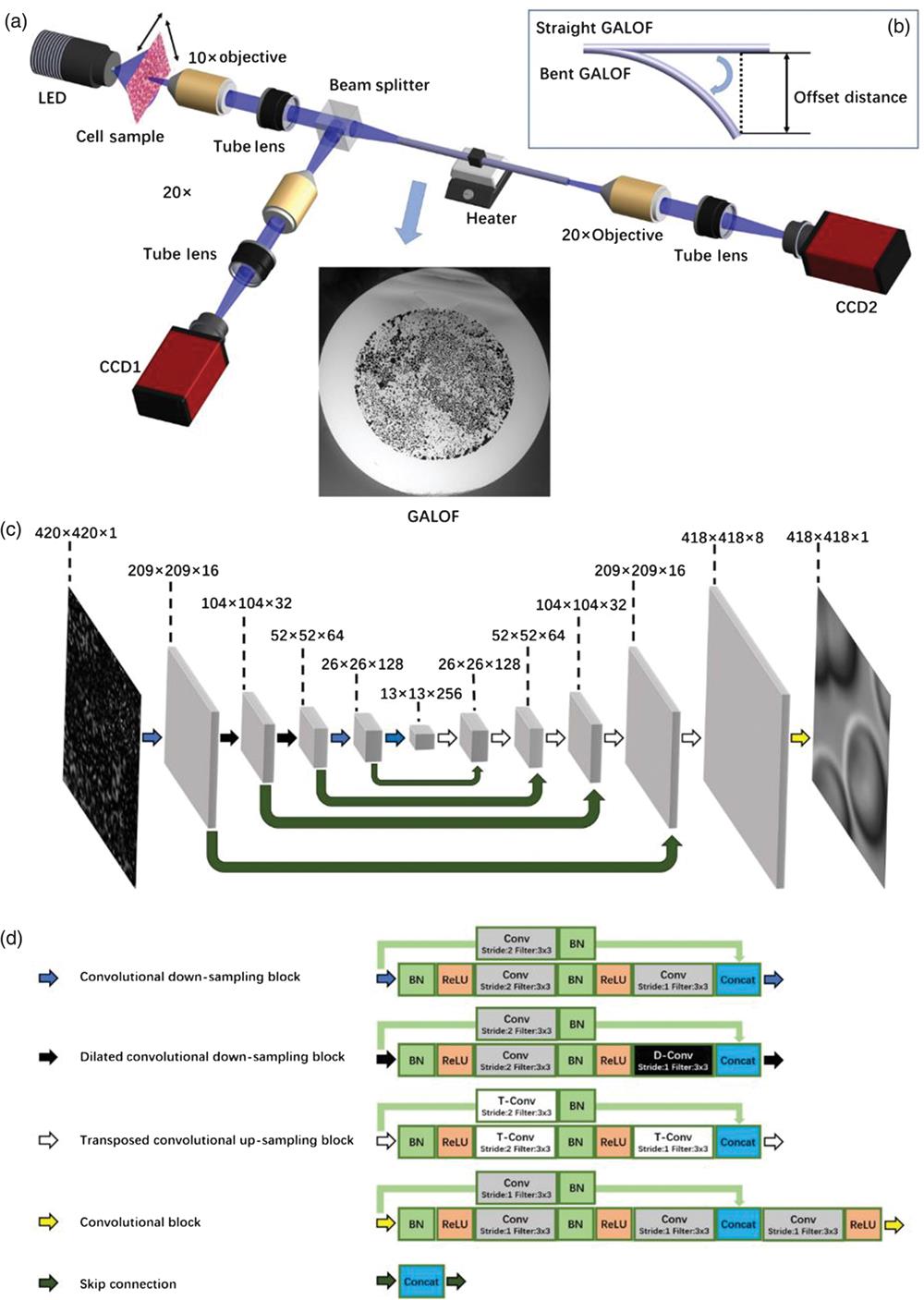
    Fig. 1. Schematic of the cell imaging setup and the architecture of the DCNN.
    Cell imaging of different types of cells: (a)–(c) test data for human red blood cells and (d)–(f) test data for cancerous human stomach cells. All data are collected with straight GALOF, at room temperature with 0-mm imaging depth. The length of the scale bar in (a1) is 4 μm. (a1)–(f1) The reference images. (a2)–(f2) The corresponding raw images. (a3)–(f3) The images recovered from the raw images. [Video S1, avi, 10 MB (URL: https://doi.org/10.1117/1.AP.1.6.066001.1)].
    Fig. 2. Cell imaging of different types of cells: (a)–(c) test data for human red blood cells and (d)–(f) test data for cancerous human stomach cells. All data are collected with straight GALOF, at room temperature with 0-mm imaging depth. The length of the scale bar in (a1) is 4  μm. (a1)–(f1) The reference images. (a2)–(f2) The corresponding raw images. (a3)–(f3) The images recovered from the raw images. [Video S1, avi, 10 MB (URL: https://doi.org/10.1117/1.AP.1.6.066001.1)].
    Multiple depth cell imaging: (a)–(f) Test data for human red blood cells. All data are collected with straight GALOF at room temperature. All three images in each column are from the same depth. The length of the scale bar in (a1) is 4 μm. (a1)–(f1) The reference images; (a2)–(f2) the corresponding raw images. The distance between the image of the object and the fiber input facet is defined as the depth. Initially, the image of the object is located at the GALOF’s input facet with 0-mm depth. Then the imaging depth is increased in steps of 1 mm by moving the fiber input end using a translation stage. As illustrated in (g), (a2)–(f2) are obtained by varying the imaging depth from 0 to 5 mm with steps of 1 mm. (a3)–(f3) The images recovered from the corresponding raw images. (h) The averaged test MAE for each depth with the standard deviation as the error bar. More sample results, including reference, raw, and recovered images, are shown in Fig. S2 in the Supplementary Material.
    Fig. 3. Multiple depth cell imaging: (a)–(f) Test data for human red blood cells. All data are collected with straight GALOF at room temperature. All three images in each column are from the same depth. The length of the scale bar in (a1) is 4  μm. (a1)–(f1) The reference images; (a2)–(f2) the corresponding raw images. The distance between the image of the object and the fiber input facet is defined as the depth. Initially, the image of the object is located at the GALOF’s input facet with 0-mm depth. Then the imaging depth is increased in steps of 1 mm by moving the fiber input end using a translation stage. As illustrated in (g), (a2)–(f2) are obtained by varying the imaging depth from 0 to 5 mm with steps of 1 mm. (a3)–(f3) The images recovered from the corresponding raw images. (h) The averaged test MAE for each depth with the standard deviation as the error bar. More sample results, including reference, raw, and recovered images, are shown in Fig. S2 in the Supplementary Material.
    Cell imaging at different temperatures. (a1)–(c1) Test raw images of human red blood cells collected at 20°C, 35°C, and 50°C, respectively. The scale bar length in (a1) is 4 μm. (a2)–(c2) Images recovered from (a1)–(c1); (a3)–(c3) the corresponding reference images. All data are collected with straight GALOF at 0-mm imaging depth. (d) The averaged test MAE for each temperature with the standard deviation as the error bar. More test sample results, including reference, raw, and recovered images, are provided in Fig. S3 in the Supplementary Material.
    Fig. 4. Cell imaging at different temperatures. (a1)–(c1) Test raw images of human red blood cells collected at 20°C, 35°C, and 50°C, respectively. The scale bar length in (a1) is 4  μm. (a2)–(c2) Images recovered from (a1)–(c1); (a3)–(c3) the corresponding reference images. All data are collected with straight GALOF at 0-mm imaging depth. (d) The averaged test MAE for each temperature with the standard deviation as the error bar. More test sample results, including reference, raw, and recovered images, are provided in Fig. S3 in the Supplementary Material.
    Cell imaging under bending. (a)–(e) Data in each column correspond to examples with the bending offset distance listed above. The definition of offset distance is illustrated in Fig. 1(b). The bending angle range corresponding to offset distances between 0 and 2 cm is about 3 deg. For more details, see Sec. 2. (a1)–(e1) Raw images collected at different bending offset distances. The scale bar length in (a1) is 4 μm. (a2)–(e2) Images reconstructed from (a1)–(e1); (a3)–(e3) the corresponding reference images. (f) Averaged test MAE for five different bending states with the standard deviation as the error bar. More sample results of human red blood cells, including reference, raw, and recovered images, are provided in Fig. S4 in the Supplementary Material.
    Fig. 5. Cell imaging under bending. (a)–(e) Data in each column correspond to examples with the bending offset distance listed above. The definition of offset distance is illustrated in Fig. 1(b). The bending angle range corresponding to offset distances between 0 and 2 cm is about 3 deg. For more details, see Sec. 2. (a1)–(e1) Raw images collected at different bending offset distances. The scale bar length in (a1) is 4  μm. (a2)–(e2) Images reconstructed from (a1)–(e1); (a3)–(e3) the corresponding reference images. (f) Averaged test MAE for five different bending states with the standard deviation as the error bar. More sample results of human red blood cells, including reference, raw, and recovered images, are provided in Fig. S4 in the Supplementary Material.
    Cell imaging transfer learning. (a)–(c) Sample cell images in the set of training data. The scale bar length in (a) is 4 μm. There are three different types of cells in the set of training data: (a) an image of human red blood cells, (b) an image of frog blood cells, and (c) an image of polymer microspheres. (d)–(f) Test process using data from images of bird blood cells. (d1)–(d4) Raw images of bird blood cells transported through straight GALOF taken at 0 mm imaging depth and at room temperature. (e1)–(e4) Images reconstructed from (d1)–(d4); (f1)–(f4) the corresponding reference images of bird blood cells. (g) Training and validation accuracy improvement curves using MAE as the metric over 80 epochs. (h) Averaged test MAE of the bird blood cell images with the standard deviation as the error bar.
    Fig. 6. Cell imaging transfer learning. (a)–(c) Sample cell images in the set of training data. The scale bar length in (a) is 4  μm. There are three different types of cells in the set of training data: (a) an image of human red blood cells, (b) an image of frog blood cells, and (c) an image of polymer microspheres. (d)–(f) Test process using data from images of bird blood cells. (d1)–(d4) Raw images of bird blood cells transported through straight GALOF taken at 0 mm imaging depth and at room temperature. (e1)–(e4) Images reconstructed from (d1)–(d4); (f1)–(f4) the corresponding reference images of bird blood cells. (g) Training and validation accuracy improvement curves using MAE as the metric over 80 epochs. (h) Averaged test MAE of the bird blood cell images with the standard deviation as the error bar.
    Jian Zhao, Yangyang Sun, Hongbo Zhu, Zheyuan Zhu, Jose E. Antonio-Lopez, Rodrigo Amezcua Correa, Shuo Pang, Axel Schulzgen. Deep-learning cell imaging through Anderson localizing optical fiber[J]. Advanced Photonics, 2019, 1(6): 066001
    Download Citation