In biomedical science and clinical applications, visualizations of real-time cell activity, morphology, and overall tissue architecture are crucial for fundamental research and medical diagnosis.^1,2 This usually requires real-time in vivo imaging to be performed in a minimally invasive way with the ability to deeply penetrate into organs or tissues. Due to their miniature size and flexible imaging transfer capability, fiber-optic imaging systems (FOISs) have been widely applied to this domain.^2–10 Current solutions encounter challenges due to poor compatibility with broadband incoherent illumination, bulky and complex distal optics, low imaging quality and speed, and extreme sensitivity to perturbations. These limitations mainly originate from both the optical fiber device and the imaging reconstruction method. For example, multicore optical fibers (MCFs) and multimode fibers (MMFs) are the two most widely used fibers in these systems. Most conventional MCF-based systems usually require extra distal optics or mechanical actuators, which limits the extent of miniaturization and induces large penetration damage.^3,8 The particular core patterns featured in MCFs result in pixelated artifacts in images transported through such fibers.^2,10–13 Even if recently reported MCF-based systems using the wavefront-shaping method can mitigate pixelated artifacts to some extent, strong core-to-core coupling in MCFs makes MCF-based FOISs inherently sensitive to deformation and rather intolerant to perturbations.^14–17 The core-to-core crosstalk in MCFs also limits the mode density and leads to the requirement of narrowband light sources for illumination in MCF-based FOISs.¹² Typical systems using MMF rely on image reconstruction processes using the transmission matrix (TM) method to compensate for randomized phases through wavefront shaping.^5,6,9,18,19 This kind of reconstruction process is vulnerable to perturbations due to the mode properties of MMFs. Minor changes of temperature (a few degrees Celsius) or slight fiber movement (a few hundred micrometers) can induce mode coupling and scramble the precalibrated transmission matrix.⁹ In addition, most state-of-the-art FOISs relying on the TM method suffer from a slow imaging speed limited by the refresh rate of wavefront-shaping devices and are not fully compatible with a broadband incoherent light source, since a coherent light source is required to perform phase-shifting interferometry.^17,20–22 The interferometry applied in such systems also results in complexity, polarization-sensitivity, and rather high levels of noise.^17,20,21

Recent burgeoning deep-learning technology and the latest discoveries of the novel properties of glass-air Anderson localizing optical fibers (GALOFs) open an avenue for overcoming these challenges and fundamentally promoting the overall performance of FOISs. Deep-learning technology is a fast-developing research field that has gained great success in imaging applications and demonstrated better performance than conventional model-based methods.^23–29 Deep convolutional neural networks (DCNNs) are very powerful techniques because they represent a universal approach to the imaging reconstruction problem.³⁰ Instead of relying on known models and priors, the DCNN directly learns the underlying physics of imaging transmission systems through a training process using a large training dataset without any advance knowledge. Deep learning is particularly suitable for the inverse imaging problem of FOISs: the trained DCNN learns the mapping function between the measured imaging data and the input imaging data; well-designed and trained DCNNs can be used to predict input images even if the particular type of images is not included in the set of training data. The application of DCNNs addresses two major bottlenecks of current FOISs. First, it is often extremely difficult to develop an accurate physics model for wave propagation through FOISs. For example, there is no analytical physics model to describe the TM of GALOFs, and numerical simulations require significant computational resources to model even simplified propagation processes.³¹ With the help of DCNNs, the TM of the whole system is learned using just a personal computer without composing a complicated physics model.³² The image mapping process is very fast, on the order of several milliseconds on regular GPUs. Second, image mapping utilizing DCNNs is only based on measurements of intensity images using conventional CCD cameras and no particular requirements are imposed on the coherence or polarization properties of the light source.^32,33 In contrast to existing methods, this could speed up the imaging process and simplify the system to a large extent while simultaneously maintaining a high-imaging quality.

The use of DCNNs for simple binary image recovery and classification after transport through optical fibers has been reported recently.^32–37 For image transmission, different types of optical fibers, MMF,^33,34,36 MCF,³⁷ and GALOF,³² have been utilized in recently reported DCNN-based FOISs. Being limited by strong-mode coupling and low-mode density, the sensitivity to temperature variation and mechanical bending and low imaging quality hinder deep-learning-based MMF or MCF systems from developing flexible endoscopy with high-quality imaging capability.^33–37 In contrast, the DCNN-GALOF system demonstrated bending-independent imaging capabilities while maintaining high imaging quality and transfer-learning capability simultaneously.³² This robust performance is based on the unique mode properties of the GALOF.^38–40 Multiple scattering in the disordered refractive index structure of the transverse plane results in modes that are localized in two-dimensional space of the GALOF cross section and can freely propagate along the axial direction of the GALOF.⁴⁰ The imaging information is encoded and transferred by thousands of densely packed transversely localized modes in the GALOF. It has been shown that the point spread function based on these modes does not degrade with propagation distance.⁴¹ Unlike MMF, most of the modes mediated by transverse Anderson localization demonstrate single-mode properties, which makes the device rather insensitive to external perturbations.^38,42 For example, the localized modes should have the potential to withstand extremely strong bending (bending radius∼0.5mm), which contrasts with the high bending sensitivity of both MCFs and MMFs.⁴³

Nevertheless, the design of the existing GALOF imaging system is based on a previous limited understanding of the localized modes in GALOFs. Hence, it is faced with several challenges limiting its practical application. First, the system only demonstrated success in imaging of low-resolution sparse objects, such as the binary MNIST handwritten numbers. There is a chasm between sparse binary object reconstruction and the reconstruction of biological objects, which are typically different types of cells or tissue with complicated morphologic features. Second, the demonstrated transfer-learning capability of the previous DCNN-GALOF system was limited to binary sparse testing objects that shared image features quite similar to those of the objects in the training data.³² For many practical applications, it would be highly desirable if the system would be able to perform transfer learning using objects that are significantly different from the training data. Third, the previous DCNN-GALOF system performs high-quality imaging under coherent laser illumination. The ability to perform imaging under incoherent broadband illumination in the fiber imaging system would be another important step toward practical applications. For example, white-light transmission cellular micrographs are already very familiar to histopathologists, and they prefer similar white light illumination for endoscopic images.⁸ Furthermore, the coherence of lasers results in speckle patterns, which often reduce the image quality. Last but not least, the high intensity of lasers light might be damaging to biological objects such as living cells and the cost of lasers is relatively high. In contrast, incoherent broadband illumination generally avoids speckle problems and the lower intensity of incoherent light sources helps to protect cells against photobleaching and phototoxicity during the imaging process. At the same time, the cost of incoherent light sources, such as LEDs, is much lower compared with laser systems. The latest research progress on mode properties of GALOFs offers a new possibility to overcome all of these barriers and enhance the system performance of FOISs. Recently, we prove that the wavefront quality of localized modes in GALOFs is close to that of an ideal fundamental Gaussian mode.⁴² Meanwhile, the mode density is orders of magnitude higher than that of MMF and MCF.⁴² Other related research further shows that localization lengths, comparable to point spread function, of localized modes are independent of wavelengths.⁴⁴ Based on these latest discoveries, the GALOF has the potential to support a high-quality imaging process using a broadband incoherent light source. In addition, DCNN itself does not raise any requirements for illumination. Therefore, it should be possible to achieve high-quality imaging of biological objects under incoherent broadband illumination using the combination of GALOFs and DCNNs.

In this work, we develop an incoherent broadband light illuminated DCNN-GALOF imaging system with the capability to image various cell structures. Within this system, a DCNN model with a design tailored to the cell imaging task is applied, and a low-cost LED works as the light source. We call the new system Cell-DCNN-GALOF. We demonstrate that it is able to transfer high-quality, artifact-free images of different types of cells in real time. We further prove that the imaging depth of this system can reach up to several millimeters without any distal optics. In addition, we show that the image reconstruction process is remarkably robust with regard to external perturbations, such as temperature variation and fiber bending. Last but not least, the transfer-learning capability of the new system is confirmed using cells of different morphologies and classes for testing. The work presented here introduces a new platform for various practical applications, such as biomedical research and clinical diagnosis. The system performance of the Cell-DCNN-GALOF is superior to state-of-the-art systems. It is also a new cornerstone for imaging research based on waveguide devices using transverse Anderson localization.

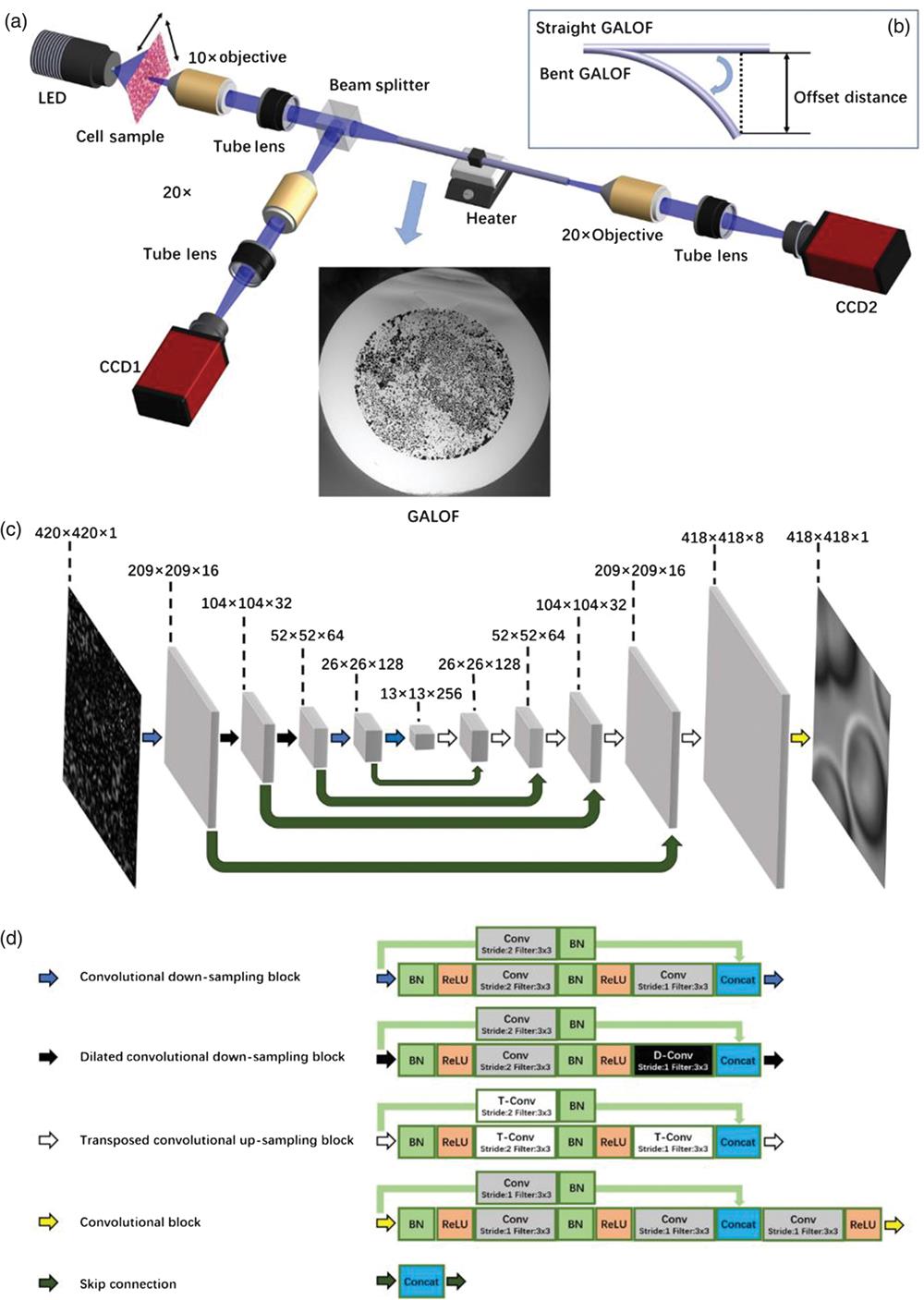
The experimental setup and details of DCNN are shown in Fig. 1. The GALOF used here is fabricated using the stack-and-draw method. Silica capillaries with different diameters and air-filling fractions are fabricated first. The outer diameter of the silica capillaries ranges from about 100 to 180μm, and the ratio of inner diameter to outer diameter ranges from 0.5 to 0.8. To make a preform, capillaries are randomly fed into a silica jacket tube. In the following steps, the preform is drawn to canes with an outer diameter around 3 mm. Finally, the cane is drawn to the GALOF with the desired size. The SEM image of the GALOF cross-section is shown in Fig. 1(a).

In Fig. 1(a), the light source is an LED with a center wavelength of 460 nm. An 80-cm long GALOF sample is utilized. The diameter of the disordered structure is about 278μm, and the air–hole-filling fraction in the disordered structure is ∼28.5%.³⁹ The numerical aperture (NA) of the GALOF, based on far-field emission angles, is measured to be ∼0.4; see Fig. S5 in the Supplementary Material. The temperature of a GALOF segment can be raised by the heater underneath. A 10-mm-long section in the middle of the GALOF is heated. We use fixed stained cell samples in all of our experiments. The images of cell samples are magnified by a 10× objective (NA = 0.3) and split into two copies sent into a reference path and a measurement path, respectively. The cell samples are scanned both vertically and horizontally with steps of 5μm to obtain training, validation, and test data sets. In the reference beam path, the image is further magnified by a 20× objective (NA=0.75) and recorded by CCD 1 (Manta G-145B, 30 fps) after passing through a tube lens. In the measurement path, the image is transported through the 80-cm-long GALOF and then projected onto CCD 2 (Manta G-145B, 30 fps) by the same combination of a 20× objective and tube lens. The reference images are labeled as the ground truth. Both reference and raw images are 8-bit grayscale images and are cropped to a size of 418×418pixels. Figure 1(b) shows that experiments are performed for both straight GALOF and bent GALOF. To bend the fiber, the input end of the GALOF is fixed, whereas the output end of the GALOF is moved by an offset distance. The amount of bending is quantified by the offset distance from the end of the bent fiber to the position of the straight fiber (equal to the length of the dashed line). The relation between the offset distance d and the corresponding bending angle of the fiber θ is given by d=L[1−cos(θ)]/θ where L is the total length of the GALOF.

Figure 1(c) shows the detailed structure of the DCNN. The raw image, which is resized to 420×420 using zero paddings, is the input layer. The input layer is decimated by five down-sampling blocks (blue and black arrows) to extract the feature maps. Then five up-sampling blocks (white arrows) and one convolutional block (yellow arrow) are applied to reconstruct the images of cell samples with a size of 418×418. To visualize the image reconstruction process, some sample feature maps are shown in Fig. S6 in the Supplementary Material. The skip connections (dark green arrows) pass feature information from feature-extraction layers to reconstruction layers by concatenation operations. The mean absolute error (MAE)-based loss metrics are calculated by comparing the reconstructed images with the reference images. The MAE is defined as |Irec−Iref|/(wh), where Irec, Iref, w, and h are the reconstructed image intensity, the reference image intensity, the width, and the height of the images, respectively. The parameters of the DCNN are optimized by minimizing the loss. Detailed block operation diagrams corresponding to the respective arrows are shown on the right side of Fig. 1(d) (BN, batch normalization; ReLU, rectified linear unit; Conv, convolution; D-Conv, dilated convolution; T-Conv, transposed convolution; concat, concatenation). The Keras framework is applied to develop the program code for the DCNN. The regularization applied in the DCNN is defined by the L2-norm. The parameters of the DCNN are initialized by a truncated normal distribution. For both training and evaluation, the MAE is utilized as the metric. The Adam optimizer is adopted to minimize the loss function. During the training process, the batch size is set at 64 and the training is run through 80 epochs with shuffling at each epoch for all of the data shown in this paper. The learning rate is set at 0.005. Both training and test processes are run in parallel on two GPUs (GeForce GTX 1080 Ti).

To demonstrate the imaging reconstruction capability, two different types of cells, human red blood cells and cancerous human stomach cells, serve as objects. By scanning across different areas of the cell sample, we collect 15,000 reference and raw images as the training set, 1000 image pairs as the validation set, and another 1000 image pairs as the test set for each type of cell. During the first data acquisition process, the GALOF is kept straight and at room temperature of about 20°C. The imaging depth is 0 mm, meaning that the image plane is located directly at the fiber input facet. The training data are loaded into the DCNN [see Fig. 1(c) for DCNN structure] to optimize the parameters of the neural network and generate a computational architecture that can accurately map the fiber-transported images to the corresponding original object. After the training process, the test data are applied to the trained model to perform imaging reconstruction and evaluate its performance using the normalized MAE as the metric. In the first round of experiments, we train and test each type of cell separately. With a training data set of 15,000 image pairs, it takes about 6.4 h to train the DCCN over 80 epochs on two GPUs using a personal computer. The accuracy improvement curves for both training and validation processes over all 80 epochs are provided in Fig. S1 in the Supplementary Material. After training, the reconstruction time of a single test image is about 0.05 s. Figure 2 shows some samples from the test data set. In Figs. 2(a)–2(c), reference images, raw images, and recovered images of three in succession collected and reconstructed images of human red cells are shown, whereas in Figs. 2(d)–2(f), three images of cancerous stomach cells are presented. Comparing the reference images with the reconstructed images, it is clear that the separately trained DCNNs are able to reconstruct images of both cell types remarkably well. The averaged normalized test MAEs are 0.024 and 0.027 for the human red blood cells and the cancerous human stomach cells, respectively, with standard deviations of 0.006 and 0.011. To further highlight the real-time imaging capability of our system, we visualize the test process for these two cell types in Video S1. This real-time imaging capability is highly desirable for many practical applications, such as in situ morphologic examinations of living tissues in their native context for pathology.

Distal optics located at the fiber input end hinders conventional FOIS from miniaturizing the size of the imaging unit. Here we are investigating the ability of our Cell-DCNN-GALOF system to image objects located at various distances from the fiber input facet without distal optics. As illustrated in Fig. 3(g), the images of cells located at different imaging planes are collected by the bare fiber input end. The depth ranges from 0 to 5 mm with steps of 1 mm. The changing of depth is performed by moving the fiber input tip. Under our experimental conditions, the defocus-enhanced phase-contrast effect⁴⁵ can be ignored due to the incoherent illumination and the stained cell samples. For each individual depth, 15,000 reference and raw images are collected as the training set, and another 1000 image pairs serve as the test set. The GALOF is kept straight and at room temperature during data collection. The DCNN is trained separately for each depth resulting in depth-specific parameters. Examining reference and reconstructed test images shown in Figs. 3(a)–3(f), high-quality image transmission and reconstruction can be achieved up to depths of at least 3 mm. The first visual degradation of the imaging quality appears around 4 mm, and the visual quality of the reconstructed images drops further at 5-mm depth. The corresponding quantitative image quality evaluation is shown in Fig. 3(h). The normalized MAE increases almost linearly with a slope of about 0.008 per mm. Based on these data, we conclude that our system can transfer high-quality cell images for objects being several mm away from the fiber input facet without the need for any distal optics. Therefore, the size of an image transmitting endoscope based on our system could be potentially minimized to the diameter of the fiber itself and the penetration damage could be reduced to a minimum without degrading the quality of the image of biological objects. The fiber could collect images of organs without touching them directly, enabling a minimally invasive, high-performance imaging system.

In practical applications, the optical fiber of the FOIS often needs to be inserted deeply into the cavity of living organs. This requires the imaging system to tolerate thermal variation and fiber bending. For MMF-based FOIS, the increase of temperature or bending of the fiber when inserting the fiber into organs or tissues induces strong variations of the mode coupling. These variations decrease the performance of MMF-based imaging systems due to induced changes of the TM.⁹ This problem can be overcome using GALOF since most of the modes embedded in GALOF show single-mode characteristics, which increase the system tolerance and can make it immune even to rather strong perturbations. We first investigate the effect of temperature variation on our Cell-DCNN-GALOF system by changing the temperature of a 10-mm-long GALOF segment with a heater. During the data collection, we keep the GALOF straight and at 0-mm imaging depth. We collect 15,000 image pairs at 20°C as the training data. For test data, we record three sets of test data where the GALOF segment is heated to 20°C, 35°C, and 50°C, respectively. Each set of test data consists of 1000 image pairs. The DCNN model is only trained utilizing the training data collected at 20°C. Subsequently, the trained model is applied to perform test image reconstruction of data acquired at all three temperatures. In Figs. 4(a)–4(c), some sample images are shown. Comparing the reference with reconstructed images, the visual imaging quality is not affected by the thermal change even for a 30°C variation. Most body temperatures of humans and animals fall into this range. This confirms the remarkable robustness of our Cell-DCNN-GALOF system regarding temperature fluctuations, which makes the system particularly suitable for in vivo imaging.

Next, we test the effect of fiber bending on the performance of our Cell-DCNN-GALOF system. We keep the temperature of the fiber at room temperature and the imaging depth at 0 mm. We collect 15,000 image pairs with straight GALOF as the training data and record five sets of separate test data corresponding to five different bending states. Each test set consists of 1000 image pairs. Experimentally, the bending is induced by moving the fiber end by a specified offset distance as illustrated in Fig. 1(b). The relation between the offset distance and the bending angle of the fiber is explained in Sec. 2. We first train the model only using the training data collected from straight GALOF. Then test images from all five different bending states are reconstructed by the nonbending-data trained DCNN model and evaluated using the MAE. The results are shown in Fig. 5. Based on the recovered images in Figs. 5(a₂)–5(e₂), high-fidelity cell imaging transfer and reconstruction could be performed without any retraining for offset distances smaller than 2 cm (a bending angle of ∼3deg). The corresponding change of the normalized averaged MAE with bending is depicted in Fig. 5(f). The MAE increases by about 0.02 for every centimeter (∼0.013perdeg) of bending. In contrast, any tiny fiber movement (a few hundred micrometers for MMF or a few millimeters for MCF) in MMF- or MCF-based systems requires access to the distal end of the fiber to recalibrate the TM.^6,9,15 For biomedical applications, the flexibility of the Cell-DCNN-GALOF system shows the potential to satisfy the imaging requirements for observing real-time neuron activity in free-behaving objects.^2,9

We have shown that our DCNN is able to perform high-fidelity image restoration when training and testing are performed with the same types of cells. In practical applications, the Cell-DCNN-GALOF system would be a more efficient and higher functionalized tool if it was able to transfer its learning capability to reconstruct different types of cells that never appeared in the set of training data. To enable transfer-learning reconstruction with high fidelity, a training dataset with high diversity would certainly be beneficial. As a proof-of-concept experiment, we apply a training set with just three different types of images. Sample images are shown in Figs. 6(a)–6(c). These are images of human red blood cells, frog blood cells, and polymer microspheres. During the recording of data for training, validation, and testing, we keep the GALOF straight and the imaging plane at 0-mm depth and at room temperature. To generate data sets for training and validation, we first collect 10,000 image pairs of human red blood cells, frog blood cells, and polymer microspheres, respectively. Subsequently, all 30,000 image pairs of the three different types are mixed randomly. We extract 28,000 image pairs from those randomly mixed images as the training dataset and 1000 image pairs as the validation dataset. To characterize the training process, the accuracy improvement curves during training and validation are tracked and shown in Fig. 6(g). Both curves show convergence to low values after about 20 epochs. The differences between the validation and the training accuracy improvement curves are very small. These characteristics indicate that our DCNN is not overfitting with respect to the training dataset.

As the test data, we record 1000 image pairs from a totally different type of cell, namely bird blood cells. The raw images of the bird blood cells obtained after passing through straight GALOF are shown in Fig. 6(d). These data are fed into the trained DCNN to perform the transfer-learning reconstruction. The reconstructed and reference images are shown in Figs. 6(e) and 6(f), respectively. To enable quantitative analysis, the averaged test MAE and its standard deviation are provided in Fig. 6(h). A visual inspection demonstrates that within the reconstructed images of bird blood cells one can clearly locate the position and orientation of the nucleus for every single cell. Being trained by a fairly limited set of training data, our DCNN is still able to approximately reconstruct complex cell objects of a totally different type. This transfer-learning capability of the Cell-DCNN-GALOF system demonstrates that the underlying physics of the imaging process is captured well by the trained DCNN and should prove beneficial for practical applications, such as real-time cell counting with a mixture of different cell types.

The system performance of an FOIS is mainly determined by the imaging processing method and the physical properties of the optical fiber. Recently developed FOISs using MMFs and MCFs heavily rely on the TM method, which requires phase-shifting interferometry and adaptive optic devices, such as spatial light modulators (SLMs) or digital micromirror devices (DMDs).^5,9,14,19 Although TM-based systems have demonstrated remarkable performance, several inherent shortcomings are associated with this approach.^17,20,22 First, TM-based systems require phase-shifting interferometry for calibration, which results in complicated configurations, vulnerability to environmental noise, and incompatibility with incoherent broadband illuminations. Second, the slow refresh rate of the wavefront-shaping device (SLM or DMD) limits the calibration and imaging speed (∼10Hz for most systems). The wavefront-shaping method using an iterative optimization algorithm without measuring the TM is even more time-consuming.¹⁵ Third, the imaging quality demonstrated by these FOISs is impaired by evident artifacts, such as defective background, ghost images, and pixelations.^9,10,16,19 Moreover, the evaluation of system performance is often based on the imaging of simple binary objects, such as numbers or letters, rather than grayscale complex biological objects, which is far from practical applications.^16,33 Finally, the physics properties of MMFs or MCFs result in various challenges in these state-of-the-art systems. Although for different mechanisms, both MMFs and MCFs require narrowband illumination for the imaging process. These types of fibers are also very sensitive to perturbations.^5,9,12,15 For instance, fiber movements of a few hundred micrometers or temperature variations of about 15°C can severely disturb the MMF-based imaging process.⁹ Although an insightful complex theoretical framework has been developed recently to predict the TM of MMFs in a straight or bent state, this model is difficult to implement in a practical system.⁴⁶ Very precise knowledge of the fiber’s parameters, such as length, refractive index distribution, and bending shape, is required. In addition, this method still necessitates an SLM resulting in problems similar to other wavefront-shaping methods.

The Cell-DCNN-GALOF system overcomes many of the abovementioned drawbacks of current FOISs through the combination of DCNN and GALOF. Regarding the image processing technique, the DCNN does not impose restrictions on coherence, bandwidth, or polarization of the light. Training and test data are intensity images recorded by conventional CCD cameras without any wavefront shaping device or interferometric measurement process. On the other hand, the unique properties of the GALOF make high-quality imaging possible. Schirmacher et al.⁴⁴ confirmed that the localization lengths of modes in transverse Anderson localizing fiber remain almost constant over a very broad spectral bandwidth of ∼500nm. This means broadband illumination does not impair the point spread function of the GALOF,⁴⁴ in contrast to MMFs and MCFs. Furthermore, unlike MCFs, the point spread function of GALOF also does not degrade with the propagation distance.⁴¹ One of the fundamental reasons for the GALOF’s potential for quality imaging is the exceptionally high-mode density. For example, our GALOF features about 10modesperμm2 at ∼600nm. This is contrasted with about 1modeperμm2 and 0.1μm2 for MMFs and MCFs under similar conditions, respectively. The rather low-mode density represents a general bottleneck to the image transmission performance of MMFs and MCFs. It should be further noted that our latest research on the GALOF demonstrates that most of the strongly localized GALOF modes have a nearly diffraction-limited wavefront and high spatial coherence.⁴² These single-mode-like characteristics of the GALOF modes together with the high-mode density are the enabling properties for the robustness of the high-quality imaging process.^38,42 Finally, we would like to point out that GALOFs are also cost-effective since it only requires undoped conventional silica material and simple two-step stack-and-draw fabrication.³² In contrast, the doped material necessary to fabricate both MMFs and MCFs leads to higher costs of such for fibers.

Due to the combination of DCNN and GALOF, the imaging system performance makes a big leap forward. High-speed (∼20Hz) artifact-free biological cell imaging is realized under broadband incoherent illumination based on a very simple, stable, and affordable system. In particular, the imaging speed is just determined by the cheap hardware of a personal computer. For the same setup as presented in this paper, an even faster speed can be easily achieved by investing in better GPUs. The demonstrated tolerances of 3-deg bending and 30°C temperature change stand for significant progress compared with other state-of-the-art systems.^9,19,33 Lensless imaging and transfer learning represent important additional improvements compared with previous systems. Using the Cell-DCNN-GALOF system, we show lensless high-quality imaging of stained biological objects that are several millimeters away. This is compared with previous FOISs that demonstrate lensless imaging with rather low imaging quality of objects at a depth of only a few hundred micrometers.^9,16 It is worth noting that the demonstrated lensless imaging capability is based on stained cell samples under incoherent illumination. For lensless imaging of unstained transparent living cells under coherent illumination, further investigations need to be performed, which is beyond the scope of this work. Regarding the transfer-learning performance, previous DCNN-based FOISs demonstrate quite limited capabilities using test objects with morphologies quite similar to that of the training objects (simple binary numbers or letters).^32,33 Reconstructing different types of cell objects that are not part of any training procedure shows the transfer-learning capability of our imaging system in practical scenarios.

Although the Cell-DCNN-GALOF system has demonstrated superior system performances, optimizations on both GALOF structure and DCNN design can potentially enhance its performance further. The current setup uses a transmission mode, whereas reflection mode operation is more suitable for practical in vivo imaging. Reflection mode operation could be implemented using illumination coupled into the GALOF proximal end and guided either by parts of the disordered structure or by separate channels integrated into the GALOF’s nondisordered cladding.^42,47 Even if the lensless imaging depth of the Cell-DCNN-GALOF system is able to satisfy lots of practical applications, extending the depth further is always desired. The imaging quality of the current system gradually reduces with increasing depth. This might be attributed to the fact that, under incoherent illumination, high-frequency features of the intensity objects are gradually lost with increasing depth, leading to a corresponding rise of the MAE. In future work, this problem might be relieved by optimizing the structural parameters of the GALOF. Perhaps the robustness of the system performance, for instance, the bending tolerance, can also be improved in next-generation Cell-DCNN-GALOF systems. Since this environmental stability is strongly related to the presence of transversally extended modes, the path to more robust performance might be further optimization of the random structure inside the GALOF with a maximized scattering in the transverse plane and, therefore, further enhanced Anderson localization. Maximizing the scattering should be achieved by adapting new materials with different refractive indices and optimizing the air–hole filling fraction and the air–hole size distribution. Enhanced Anderson localization creates transverse localization sites with smaller radii and fewer variations.^31,42,48 Finally, more universal transfer-learning imaging can be achieved using training data with larger diversity. However, generating highly diverse biological training data for an FOIS remains a formidable practical challenge, and the computational power available to process large amounts of training data is often an additional bottleneck. We believe that these challenges can be addressed in next-generation FIOSs for biological objects with the help of further optimized DCNN architectures.

In conclusion, it is the combination of unique GALOF properties and tailored DCNN design that enables the remarkable capabilities of the presented Cell-DCNN-GALOF imaging system. Both components, GALOF design and DCNN architecture, still have room for improvements, and future research will consider both components and their interplay. We are very optimistic that the presented architecture can be the basis for future high-fidelity imaging systems that are minimally invasive and demonstrate robust performance in dynamic environments.

References

[1] F. Koenig, J. Knittel, H. Stepp. Diagnosing cancer in vivo. Science, 292, 1401-1403(2001).
[2] V. Szabo et al. Spatially selective holographic photoactivation and functional fluorescence imaging in freely behaving mice with a fiberscope. Neuron, 84, 1157-1169(2014).
[3] B. A. Flusberg et al. Fiber-optic fluorescence imaging. Nat. Methods, 2, 941-950(2005).
[4] T. J. Muldoon et al. Subcellular-resolution molecular imaging within living tissue by fiber microendoscopy. Opt. Express, 15, 16413-16423(2007).
[5] T. Cizmar, K. Dholakia. Exploiting multimode waveguides for pure fibre-based imaging. Nat. Commun., 3, 1027(2012).
[6] Y. Choi et al. Scanner-free and wide-field endoscopic imaging by using a single multimode optical fiber. Phys. Rev. Lett., 109, 203901(2012).
[7] I. N. Papadopoulos et al. High-resolution, lensless endoscope based on digital scanning through a multimode optical fiber. Biomed. Opt. Express, 4, 260-270(2013).
[8] M. Hughes, T. P. Chang, G.-Z. Yang. Fiber bundle endocytoscopy. Biomed. Opt. Express, 4, 2781-2794(2013).
[9] S. Ohayon et al. Minimally invasive multimode optical fiber microendoscope for deep brain fluorescence imaging. Biomed. Opt. Express, 9, 1492-1509(2018).
[10] Y. Chang et al. Compact high-resolution endomicroscopy based on fiber bundles and image stitching. Opt. Lett., 43, 4168-4171(2018).
[11] K. L. Reichenbach, C. Xu. Numerical analysis of light propagation in image fibers or coherent fiber bundles. Opt. Express, 15, 2151-2165(2007).
[12] X. Chen, K. L. Reichenbach, C. Xu. Experimental and theoretical analysis of core-to-core coupling on fiber bundle imaging. Opt. Express, 16, 21598-21607(2008).
[13] J. M. Stone et al. Low index contrast imaging fibers. Opt. Lett., 42, 1484-1487(2017).
[14] D. Kim et al. Toward a miniature endomicroscope: pixelation-free and diffraction-limited imaging through a fiber bundle. Opt. Lett., 39, 1921-1924(2014).
[15] U. Weiss, O. Katz. Two-photon lensless micro-endoscopy with in-situ wavefront correction. Opt. Express, 26, 28808-28817(2018).
[16] V. Tsvirkun et al. Widefield lensless endoscopy with a multicore fiber. Opt. Lett., 41, 4771-4774(2016).
[17] E. R. Andresen et al. Ultrathin Endoscopes Based on Multicore Fibers and Adaptive Optics: A Status Review and Perspectives(2016).
[18] T. Čižmár, K. Dholakia. Shaping the light transmission through a multimode optical fibre: complex transformation analysis and applications in biophotonics. Opt. Express, 19, 18871-18884(2011).
[19] S. Turtaev et al. High-fidelity multimode fibre-based endoscopy for deep brain in vivo imaging. Light Sci. Appl., 7, 92(2018).
[20] S. M. Popoff et al. Controlling light through optical disordered media: transmission matrix approach. New J. Phys., 13, 123021(2011).
[21] S. M. Popoff et al. Measuring the transmission matrix in optics: an approach to the study and control of light propagation in disordered media. Phys. Rev. Lett., 104, 100601(2010).
[22] H. Yu et al. Recent advances in wavefront shaping techniques for biomedical applications. Curr. Appl Phys., 15, 632-641(2015).
[23] Y. Rivenson et al. Deep learning microscopy. Optica, 4, 1437-1443(2017).
[24] S. Li et al. Imaging through glass diffusers using densely connected convolutional networks. Optica, 5, 803-813(2018).
[25] Y. Li, Y. Xue, L. Tian. Deep speckle correlation: a deep learning approach toward scalable imaging through scattering media. Optica, 5, 1181-1190(2018).
[26] Y. Rivenson et al. Virtual histological staining of unlabelled tissue-autofluorescence images via deep learning. Nat. Biomed. Eng., 3, 466-477(2019).
[27] Y. Xue et al. Reliable deep-learning-based phase imaging with uncertainty quantification. Optica, 6, 618-629(2019).
[28] H. Pinkard et al. Deep learning for single-shot autofocus microscopy. Optica, 6, 794-797(2019).
[29] J. Zhao et al. A path to high-quality imaging through disordered optical fibers: a review. Appl. Opt., 58, D50-D60(2019).
[30] M. T. McCann, K. H. Jin, M. Unser. Convolutional neural networks for inverse problems in imaging: a review. IEEE Signal Process. Mag., 34, 85-95(2017).
[31] S. Karbasi et al. Detailed investigation of the impact of the fiber design parameters on the transverse Anderson localization of light in disordered optical fibers. Opt. Express, 20, 18692-18706(2012).
[32] J. Zhao et al. Deep learning imaging through fully-flexible glass-air disordered fiber. ACS Photonics, 5, 3930-3935(2018).
[33] B. Rahmani et al. Multimode optical fiber transmission with a deep learning network. Light Sci. Appl., 7, 69(2018).
[34] N. Borhani et al. Learning to see through multimode fibers. Optica, 5, 960-966(2018).
[35] P. Wang, J. Di. Deep learning-based object classification through multimode fiber via a CNN-architecture SpeckleNet. Appl. Opt., 57, 8258-8263(2018).
[36] U. Kürüm et al. Deep learning enabled real time speckle recognition and hyperspectral imaging using a multimode fiber array. Opt. Express, 27, 20965-20979(2019).
[37] J. Shao et al. Fiber bundle image restoration using deep learning. Opt. Lett., 44, 1080-1083(2019).
[38] G. Ruocco et al. Disorder-induced single-mode transmission. Nat. Commun., 8, 14571(2017).
[39] J. Zhao et al. Image transport through meter-long randomly disordered silica-air optical fiber. Sci. Rep., 8, 3065(2018).
[40] A. Mafi. Transverse Anderson localization of light: a tutorial. Adv. Opt. Photonics, 7, 459-515(2015).
[41] S. Karbasi, K. W. Koch, A. Mafi. Image transport quality can be improved in disordered waveguides. Opt. Commun., 311, 72-76(2013).
[42] B. Abaie et al. Disorder-induced high-quality wavefront in an Anderson localizing optical fiber. Optica, 5, 984-987(2018).
[43] S. Karbasi, K. W. Koch, A. Mafi. Multiple-beam propagation in an Anderson localized optical fiber. Opt. Express, 21, 305-313(2013).
[44] W. Schirmacher et al. What is the right theory for Anderson localization of light? An experimental test. Phys. Rev. Lett., 120, 067401(2018).
[45] C. J. R. Sheppard. Defocused transfer function for a partially coherent microscope and application to phase retrieval. J. Opt. Soc. Am. A, 21, 828-831(2004).
[46] M. Plöschner, T. Tyc, T. Čižmár. Seeing through chaos in multimode fibres. Nat. Photonics, 9, 529-535(2015).
[47] A. Mafi et al. Disordered Anderson localization optical fibers for image transport—a review. J. Lightwave Technol.(2019). https://doi.org/10.1109/JLT.2019.2916020
[48] S. Karbasi, K. W. Koch, A. Mafi. Modal perspective on the transverse Anderson localization of light in disordered optical lattices. J. Opt. Soc. Am. B, 30, 1452-1461(2013).