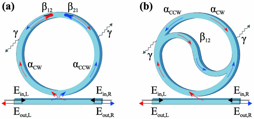
Fig. 1. Sketch of (a) ring and (b) taiji microresonator coupled to a bus waveguide. The arrows indicate the propagating fields. Specifically, the red (blue) highlights propagation in the clockwise (counter-clockwise) direction. The different symbols are defined in the text.

Fig. 2. Theoretical results for a Hermitian coupling. Panels (a1) and (a2) show the transmission and reflection spectra for an excitation from the left and right input, respectively. Maps (b1) and (b2) show, respectively, the right and left output field intensities as a function of the angle (θh) and of the detuning frequency (Δω) for a symmetric interferometric excitation in units of mW·Hz. Panels (c1) and (c2) show the output field spectral lineshapes for fixed values of θh={±π,π/4,π/2,−π/2}. The red (blue) lines denote the left (right) output fields. The graph (d) shows the modulus of the inner product of the eigenstates and their real and imaginary parts as a function of θh. The solid-black, solid-orange, and dashed-magenta lines refer to |⟨v1|v2⟩|, |⟨ℑ[v1]|ℑ[v2]⟩|, and |⟨ℜ[v1]|ℜ[v2]⟩|, respectively. The coupling is Hermitian, and therefore the two eigenstates are orthogonal, i.e., ⟨v1|v2⟩=0. Here, we used the following coefficients: Γ=γ=6.8  GHz, β12=−β21*=33.2  GHz, and ω0=2π·193  THz.

Fig. 3. Theoretical results for a non-Hermitian coupling. The transmitted and reflected intensities are shown in panels (a1) and (a2), for left (εin,L=1mW·Hz and εin,R=0) or right (εin,L=0 and εin,R=1mW·Hz) input. The blue (red) curves denote the right (left) output fields. Panels (b1) and (b2) show the intensity of the output fields as a function of the angle θ and frequency detuning Δω for a symmetric interferometric excitation (εin,L=εin,R=1mW·Hz) in units of mW·Hz. (c1)–(c4) Spectral output field intensities for few θ values given in each panel. (d) Modulus of the eigenstate inner product. The non-Hermitian nature of the coupling makes the eigenstates non-orthogonal, i.e., ⟨v1|v2⟩≠0. Here, we used the following coefficients: Γ=γ=6.8  GHz, β12=20.2  GHz, β21=(−20.2+9i)  GHz, and ω0=2π·193  THz.

Fig. 4. Theoretical results for an asymmetric interferometric excitation which satisfies Eq. (13). Panels (b1) and (b2) show the intensities of the output fields as a function of the angle θ and frequency detuning Δω in units of mW·Hz. The graphs (b1) and (b2) show the spectral output field intensities for θ=π/2 and θ=−π/2, respectively. Here, we used the same coefficients as in Fig. 3, i.e., Γ=γ=6.8  GHz, β12=20.2  GHz, β21=(−20.2+9i)  GHz, and ω0=2π·193  THz.

Fig. 5. Theoretical results for a taiji microresonator coupled to a bus waveguide. Panels (a1) and (a2) show the transmitted and reflected intensities as a function of the frequency detuning Δω at the left and right outputs, respectively. The blue (red) curves refer to the output fields from the right (left) waveguide edges. The maps (b1) and (b2) show the intensities of the output fields as a function of the phase ϕ and Δω for a symmetric interferometric excitation in units of mW·Hz. The transmitted spectral intensities are plotted on the graphs (c1)–(c4) for ϕ=−π/2, 3π/4, ±π, and 0, respectively. The graph (d) shows the modulus of the inner product of the eigenstates. As expected, the taiji works on an exceptional point, and therefore the eigenstates are parallel, i.e., ⟨v1|v2⟩=1. Here, we used the following coefficients: Γ=γ=6.8  GHz, β12=12  GHz<2γ, β21=0, and ω0=2π·193  THz.

Fig. 6. Sketch of the experimental setup. PC, personal computer to control the instruments; CWTL, continuous wave tunable laser to excite the system; OI, optical isolator to protect the laser from back-reflections; FS, fiber splitter to split the signal; VOA, variable optical attenuator to control the amplitudes; FPC, fiber polarization controller to set the transverse electric polarization at the chip grating couplers; DL, delay line to balance the two optical paths; OC, optical circulator to measure and excite simultaneously the counter-propagating fields; PD, photo detector, and PicoScope, PC oscilloscope, to measure the output powers; AS, alignment stage, and IRC, infrared camera, to see and align the stripped fibers with the sample.

Fig. 7. Experimental results for a microring. Panels (a1) and (a2) show the transmitted and reflected intensities as a function of the frequency detuning (Δω) for the right and left excitations. Panels (b1) and (b2) display the doublet splitting (δω=ω</>−ω0) for a symmetric interferometric excitation as a function of the phase θ for the right or left output fields. ω</> are the measured frequency minima of the doublet. The magenta (purple) dots refer to δω=ω<−ω0 for the right (left) output fields. The black (gray) squares refer to δω=ω>−ω0 for the right (left) output fields. The dashed magenta (purple) and dash-dotted black (gray) curves show the theoretical results modeled using the fitting parameters of the one-side excitation. Panels (c1), (c2), (c3), and (c4) show the output field intensities as a function of Δω for θ=0.73π, −0.74π, 0.48π, and −0.52π, respectively. The blue (red) curves refer to the right (left) output field intensities. The dashed-black and dotted-black lines are the fit with the theoretical model for the right and left output fields, respectively. From the fit we obtain the following coefficients: Γ=2.662±0.003  GHz, γ=4.56±0.01  GHz, β12=(−19.72±0.02)−i(0.2±0.4) GHz, and β21=(20.67±0.02)+i(0.8±0.4)  GHz.

Fig. 8. Experimental results for a taiji microresonator. The red (blue) curves refer to the left (right) output field. The dashed and dash-dotted black lines show the fit with the theoretical model. Panels (a1) and (a2) show the output fields as a function of the frequency detuning Δω for a left and right excitation, respectively. Panels (b1) and (b2) display the doublet splitting (δω=ω</>−ω0) for a symmetric interferometric excitation as a function of the phase ϕ for the right or left output fields. ω</> are the measured frequency minima of the doublet. The magenta (purple) dots refer to δω=ω<−ω0 for the right (left) output fields. The black (gray) squares refer to δω=ω>−ω0 for the right (left) output fields. The dashed magenta (purple) and dash-dotted black (gray) curves show the theoretical results modeled by using the fitting parameters of the one-side excitation. Panels (c1) and (c2) show two examples of spectra for an interferometric excitation with a phase ϕ=0.93π and −0.35π, respectively. From the fit, we obtain the following coefficients: Γ=75.1±0.1  GHz, γ=42.6±0.1  GHz, β12=(−90.8±0.1)−i(24.17±0.03)  GHz, β21=(8.7±0.1)−i(7.30±0.09)  GHz.

Table 1. Real and Imaginary Parts of the Microresonator’s Eigenvalues^a