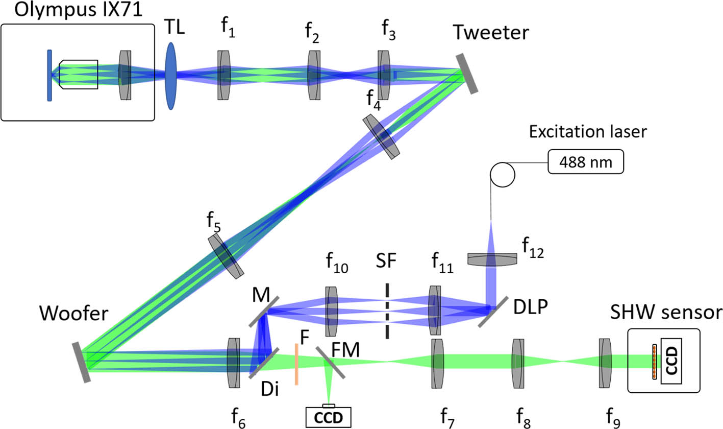
Fig. 1. Layout of the woofer–tweeter AOSIM. The DLP with 608×684 pixels (DLP3000 Texas Instruments) is placed at a conjugate plane of the objective lens focal plane. The SHW sensor consists of a lenslet array (f=24  mm) and a CCD camera (Photometrics) and is placed at a conjugate plane of the objective lens aperture plane. Blue line, 488 nm excitation light path (488 nm excitation laser from Spectra-Physics); green line, 515 nm emission path. The focal lengths of the lenses are f1=120  mm, f2=125  mm, f3=120  mm, f4=150  mm, f5=500  mm, f6=750  mm, f7=150  mm, f8=75  mm, f9=100  mm, f10=450  mm, f11=150  mm, f12=50  mm. M, mirror; SF, spatial filter; TL, trial lens (cylinder); F, filter; Di, dichroic mirror; FM, flip mirror.

Fig. 2. Comparison of (a)–(d) widefield and (e)–(h) SIM microscope images with and without wavefront correction. The figure shows the images of nanoparticles (110 nm) after introducing trial lens in between lenses f1 and f2. (a), (e) Without AO correction; (b), (f) woofer-only correction; (c), (d) tweeter-only correction; (d), (h) both woofer and tweeter correction. The scale bar is 5 μm.

Fig. 3. Zernike modes of the wavefront errors with and without woofer–tweeter correction. The inset is the value of the remaining Zernike modes after removing the sixth-order vertical astigmatism. The Zernike order is in Noll single-index order [43].

Fig. 4. Comparison of 0.11 μm beads under AO widefield (black line) and AOSIM (red line), Shown as line plots of the intensity of beads in areas 1 and 2 of Figs. 2(d) and 2(h). (a) Intensity profile of two closely spaced beads. The distance between two well-resolved peaks in AOSIM is 145 nm. (b) The FWHMs of a single bead in widefield and AOSIM are 235 and 140 nm, respectively.

Fig. 5. Images of GFP-labeled aCC/RP2 motoneurons of a Drosophila embryo. (a) Widefield without AO, (b) SIM without AO, (c) widefield with AO, (d) SIM with AO, (e) intensity plots of the line profiles in (a)–(d). The lines are along the dendrites of the aCC. The scale bar is 10 μm.

Fig. 6. Zernike modes of the Drosophila embryo wavefront errors with and without woofer–tweeter correction [43].

Table 1. Analysis of Measured Wavefront of Figs. 2(a)–2(d)^a