• Photonics Research
  • Vol. 10, Issue 2, 524 (2022)
Eva A. A. Pogna1, Alessandra Di Gaspare1, Kimberly Reichel1, Chiara Liberatore1, Harvey E. Beere2, David A. Ritchie2, and Miriam S. Vitiello1、*
Author Affiliations
  • 1NEST, CNR-Istituto Nanoscienze—Scuola Normale Superiore, 56127 Pisa, Italy
  • 2Cavendish Laboratory, University of Cambridge, Cambridge CB3 0HE, UK
  • show less
    DOI: 10.1364/PRJ.440463 Cite this Article Set citation alerts
    Eva A. A. Pogna, Alessandra Di Gaspare, Kimberly Reichel, Chiara Liberatore, Harvey E. Beere, David A. Ritchie, Miriam S. Vitiello. Spatial coherence of electrically pumped random terahertz lasers[J]. Photonics Research, 2022, 10(2): 524 Copy Citation Text show less
    (a) Coherence property of a light source that from being totally incoherent can be made spatially coherent by spatial filtering with a small aperture, and temporally coherent with a spectral filter. (b) Random distribution of scattering centers in random THz QCLs (gray holes) that provide optical feedback (colored arrows) and act as light out-couplers for multimode emission. (c) Scanning electron microscope image of a random THz QCL showing the hole pattern and irregular edges made to suppress Fabry–Perot modes. Scale bar corresponds to 50 μm. (d)–(f) Far-field intensity patterns of three random THz QCLs named (d) A, (e) B, and (f) C having different r/as ratios, measured at 80% of their total peak power.
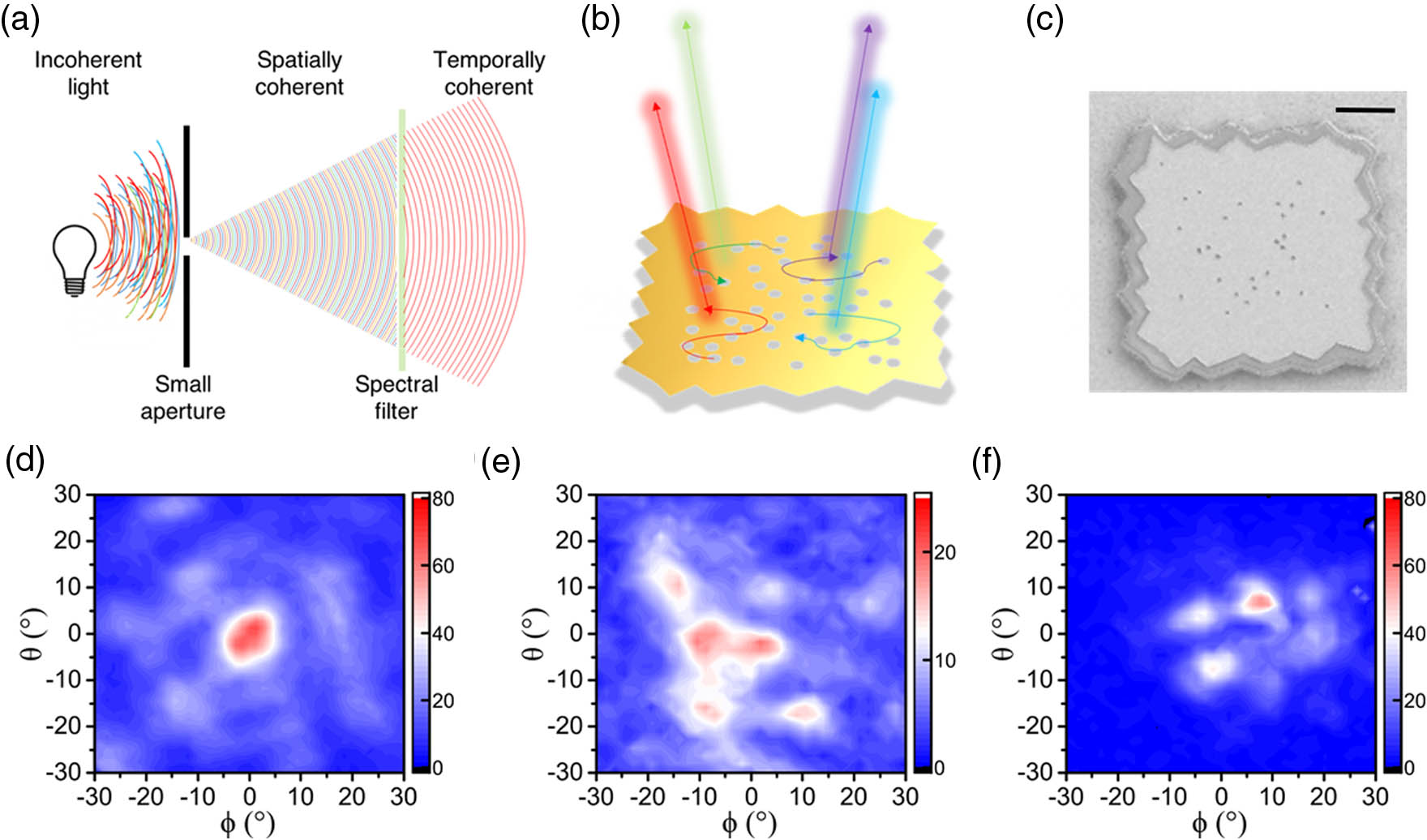
    Fig. 1. (a) Coherence property of a light source that from being totally incoherent can be made spatially coherent by spatial filtering with a small aperture, and temporally coherent with a spectral filter. (b) Random distribution of scattering centers in random THz QCLs (gray holes) that provide optical feedback (colored arrows) and act as light out-couplers for multimode emission. (c) Scanning electron microscope image of a random THz QCL showing the hole pattern and irregular edges made to suppress Fabry–Perot modes. Scale bar corresponds to 50 μm. (d)–(f) Far-field intensity patterns of three random THz QCLs named (d) A, (e) B, and (f) C having different r/as ratios, measured at 80% of their total peak power.
    (a) Schematics of the experimental setup for modified Young’s double-slit experiment. (b), (c) From top to bottom, interference patterns of samples A, B, and C acquired by placing the slits (b) parallel to the optical table or (c) orthogonal to the optical table. The noise levels are 7, 6, and 2×10⁻¹ for lasers A, B, and C, respectively, estimated as average intensity over a 10×10 pixels dark region. (d), (e) Average cross-section intensity distribution evaluated from maps in (b) and in (c) considering two pixels (colored curves) or 30 pixels (black solid line). (f) Spatial coherence value evaluated from the visibility of the fringes in (d) and (e) obtained with a horizontal (H, right panel) or vertical (V, left panel) orientation of the slits, as a function of the vertical coordinate Y (colored open dots) and compared to the values obtained in an FP THz QCL (dashed black line).
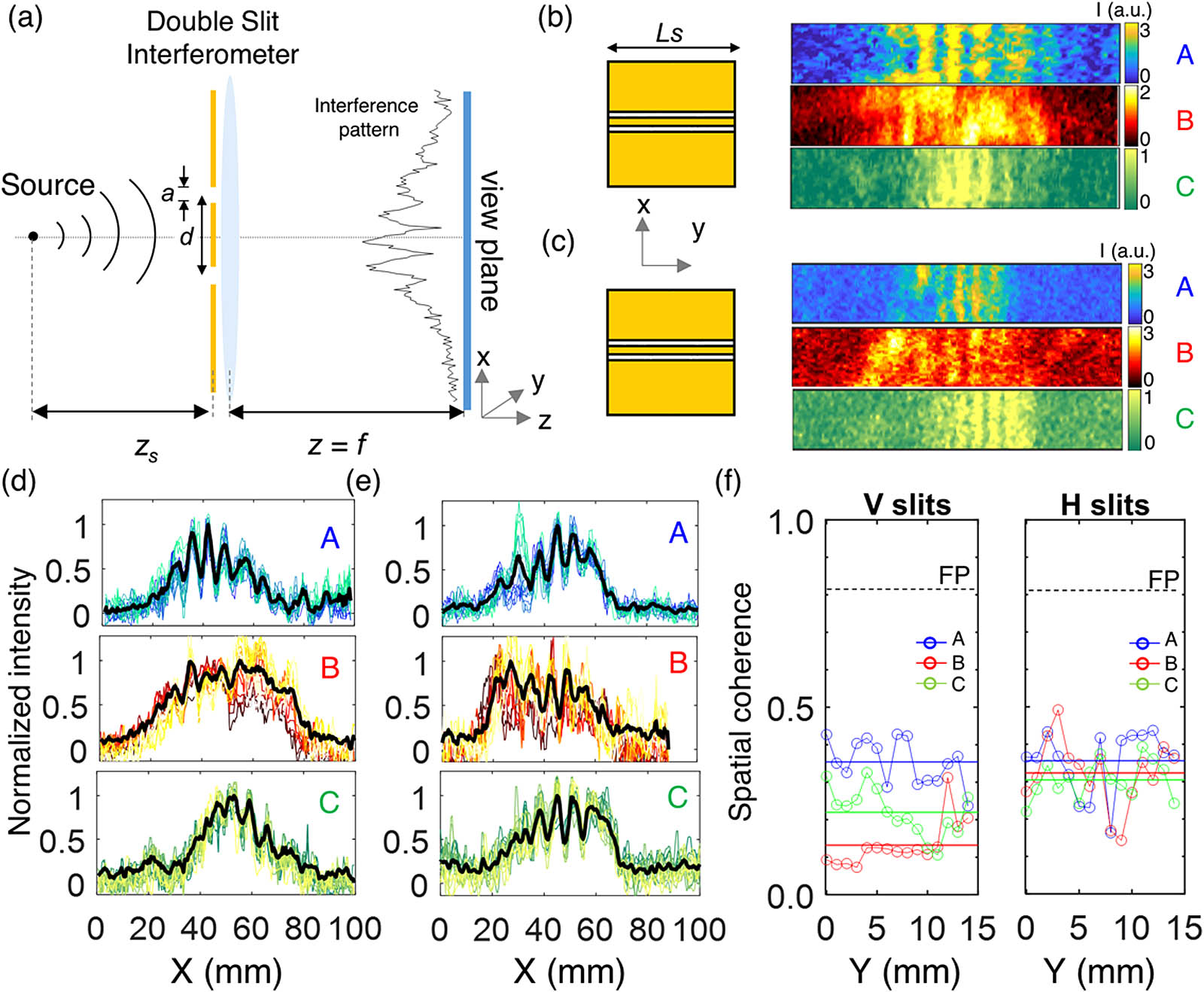
    Fig. 2. (a) Schematics of the experimental setup for modified Young’s double-slit experiment. (b), (c) From top to bottom, interference patterns of samples A, B, and C acquired by placing the slits (b) parallel to the optical table or (c) orthogonal to the optical table. The noise levels are 7, 6, and 2×101 for lasers A, B, and C, respectively, estimated as average intensity over a 10×10  pixels dark region. (d), (e) Average cross-section intensity distribution evaluated from maps in (b) and in (c) considering two pixels (colored curves) or 30 pixels (black solid line). (f) Spatial coherence value evaluated from the visibility of the fringes in (d) and (e) obtained with a horizontal (H, right panel) or vertical (V, left panel) orientation of the slits, as a function of the vertical coordinate Y (colored open dots) and compared to the values obtained in an FP THz QCL (dashed black line).
    (a) Experimental setup for confocal imaging based on random THz QCLs. (b) Photo of the maple seed we used to test our imaging setup; scale bar corresponds to 5 mm. (c) Transmission images of the sample acquired with sample A (panels on the left) and sample B (panels on the right) with open (top panels) and closed pinholes (bottom panels). The brightness of all the images is normalized for better comparison. Histogram reporting the distribution of pixel intensity around the average value ⟨I⟩ calculated for the images in (c) with open (gray) and closed pinholes (red) for samples (d) A and (e) B.
    Fig. 3. (a) Experimental setup for confocal imaging based on random THz QCLs. (b) Photo of the maple seed we used to test our imaging setup; scale bar corresponds to 5 mm. (c) Transmission images of the sample acquired with sample A (panels on the left) and sample B (panels on the right) with open (top panels) and closed pinholes (bottom panels). The brightness of all the images is normalized for better comparison. Histogram reporting the distribution of pixel intensity around the average value I calculated for the images in (c) with open (gray) and closed pinholes (red) for samples (d) A and (e) B.
    (a) Transmission images of a 2 cm×2 cm (100×100 pixels) lint-free paper tissue measured with sample C with (a) open and (b) closed pinholes. (c) Histogram reporting the distribution of pixel intensity around the average value ⟨I⟩ calculated for the images in (a), (b) with open (gray) and closed pinholes (red).
    Fig. 4. (a) Transmission images of a 2cm×2  cm (100×100  pixels) lint-free paper tissue measured with sample C with (a) open and (b) closed pinholes. (c) Histogram reporting the distribution of pixel intensity around the average value I calculated for the images in (a), (b) with open (gray) and closed pinholes (red).
    (a) Resolution test chart made by evaporating 7 nm/40 nm Cr/au on a SiO2/Si slide. (b), (c) THz transmission images of the test chart acquired with (b) FP laser and (c) sample A. (d) Contrast-to-noise ratio (CNR) evaluated from the analysis of 18 Ronchi rulers in the images acquired with the FP and random lasers, in (b) and (c), respectively. (e) Speckle contrast of the images acquired with sample A as a function of pinhole diameter. (f) Spatial resolution of the images acquired with sample A as a function of pinhole diameter. Images from which the data in (e) and (f) are extracted can be found in Appendix E.
    Fig. 5. (a) Resolution test chart made by evaporating 7 nm/40 nm Cr/au on a SiO2/Si slide. (b), (c) THz transmission images of the test chart acquired with (b) FP laser and (c) sample A. (d) Contrast-to-noise ratio (CNR) evaluated from the analysis of 18 Ronchi rulers in the images acquired with the FP and random lasers, in (b) and (c), respectively. (e) Speckle contrast of the images acquired with sample A as a function of pinhole diameter. (f) Spatial resolution of the images acquired with sample A as a function of pinhole diameter. Images from which the data in (e) and (f) are extracted can be found in Appendix E.
    Random pattern of surface holes in samples (a) A, (b) B, and (c) C, and (d) spatial autocorrelation function in the three cases evaluated as in Refs. [28,37]. The patterns and autocorrelation function for samples A and B are also reported in Ref. [37].
    Fig. 6. Random pattern of surface holes in samples (a) A, (b) B, and (c) C, and (d) spatial autocorrelation function in the three cases evaluated as in Refs. [28,37]. The patterns and autocorrelation function for samples A and B are also reported in Ref. [37].
    (a) Voltage–current density and light–current density characteristics of samples A, B, and C measured driving the devices in pulsed mode with a pulse width of 10 μs (duty cycle 10%) at a heat sink temperature of 15 K. The black star symbols indicate the operating currents at which the double-slit experiments are performed. (b)–(d) FTIR spectra of samples (b) A, (c) B, and (d) C, measured at the current densities indicated by black star symbols in (a).
    Fig. 7. (a) Voltage–current density and light–current density characteristics of samples A, B, and C measured driving the devices in pulsed mode with a pulse width of 10 μs (duty cycle 10%) at a heat sink temperature of 15 K. The black star symbols indicate the operating currents at which the double-slit experiments are performed. (b)–(d) FTIR spectra of samples (b) A, (c) B, and (d) C, measured at the current densities indicated by black star symbols in (a).
    Polar plot of laser intensity as a function of polarization angle α for samples (a) A, (b) B, and (c) C measured filtering the emission with a linear polarizer placed just before the pyroelectric detector.
    Fig. 8. Polar plot of laser intensity as a function of polarization angle α for samples (a) A, (b) B, and (c) C measured filtering the emission with a linear polarizer placed just before the pyroelectric detector.
    Interference fringes of an FP THz QCL performing a modified Young’s double-slit experiment. (a) Map of the 20 mm×85 mm region scanned with the pyroelectric detector; (b) cross-section average intensity of the map in (a) showing interference fringes.
    Fig. 9. Interference fringes of an FP THz QCL performing a modified Young’s double-slit experiment. (a) Map of the 20mm×85  mm region scanned with the pyroelectric detector; (b) cross-section average intensity of the map in (a) showing interference fringes.
    (a) Continuous wave current-voltage-power characteristics of an FP THz QCL. (b) Normalized Fourier transform infrared (FTIR) emission spectrum of the FP THz QCL, measured at J=365 A/cm2.
    Fig. 10. (a) Continuous wave current-voltage-power characteristics of an FP THz QCL. (b) Normalized Fourier transform infrared (FTIR) emission spectrum of the FP THz QCL, measured at J=365  A/cm2.
    Far-field intensity pattern of FP THz QCL, measured at I=657 mA (J=365 A/cm2).
    Fig. 11. Far-field intensity pattern of FP THz QCL, measured at I=657  mA (J=365  A/cm2).
    THz transmission image of a maple seed obtained using sample C driven at JC=549 A/cm2 (a) without inserting the pinhole and (b) with the pinhole. Images are normalized for comparison. (c) Distribution of pixel intensities around the average value ⟨I⟩ of the image with open pinhole (gray histogram) from (a), and with closed pinhole (red histogram) from (b).
    Fig. 12. THz transmission image of a maple seed obtained using sample C driven at JC=549  A/cm2 (a) without inserting the pinhole and (b) with the pinhole. Images are normalized for comparison. (c) Distribution of pixel intensities around the average value I of the image with open pinhole (gray histogram) from (a), and with closed pinhole (red histogram) from (b).
    Comparison of THz images of a test chart acquired with sample A, as it is and after filtering its emission with a pinhole of diameters ranging from 3 mm to 1 mm, as indicated in the image title.
    Fig. 13. Comparison of THz images of a test chart acquired with sample A, as it is and after filtering its emission with a pinhole of diameters ranging from 3 mm to 1 mm, as indicated in the image title.
    Linecuts of maps in Fig. 13 at the edge of the open squared feature of the test chart. Data are reported as colored dots; fits with the edge function described in the text to evaluate the spatial resolution of the images are shown as solid colored lines.
    Fig. 14. Linecuts of maps in Fig. 13 at the edge of the open squared feature of the test chart. Data are reported as colored dots; fits with the edge function described in the text to evaluate the spatial resolution of the images are shown as solid colored lines.
    Eva A. A. Pogna, Alessandra Di Gaspare, Kimberly Reichel, Chiara Liberatore, Harvey E. Beere, David A. Ritchie, Miriam S. Vitiello. Spatial coherence of electrically pumped random terahertz lasers[J]. Photonics Research, 2022, 10(2): 524
    Download Citation