Spatial coherence of electrically pumped random terahertz lasers

Eva A. A. Pogna; Alessandra Di Gaspare; Kimberly Reichel; Chiara Liberatore; Harvey E. Beere; David A. Ritchie; Miriam S. Vitiello

doi:10.1364/PRJ.440463

Abstract

Light sources with high radiance and tailored coherence properties are highly desirable for imaging applications in the mid-infrared and terahertz (THz) spectral regions, which host a large variety of molecular absorptions and distinctive fingerprints to be exploited for sensing and tomography. Here, we characterize the spatial coherence of random multimode THz quantum cascade lasers (QCLs) emitting > mW optical power per mode and showing low divergence (10°–30°), performing a modified Young’s double-slit experiment. Partial spatial coherence values ranging between 0.16 and 0.34 are retrieved, depending on the specific degree of disorder. These values are significantly lower than those (0.82) of conventional Fabry–Perot THz QCLs exploiting an identical active region quantum design. We then incorporate the devised low spatial coherence random lasers into a confocal imaging system with micrometer spatial resolution and demonstrate notable imaging performances, at THz frequencies, against spatial cross talk and speckles.

1. INTRODUCTION

Spatial coherence is a fundamental property of laser radiation that allows light focusing to diffraction limited volumes and beam propagation over long distances with minimal divergence [1]. Accounting for the phase relation between distinct points of the wavefront, the spatial coherence defines the ability of light to interfere and be diffracted. Accordingly, a high spatial coherence can be detrimental for common imaging applications, producing coherent artifacts due to interference during image formation, such as speckle patterns and diffraction fringes at sharp edges [2]. On the other hand, there are imaging techniques that require a highly coherent beam, such as holography [3], which exploits the coherent superposition of optical fields to fully reconstruct the wavefront and needs both spatial and temporal coherence for producing sharp images [4].

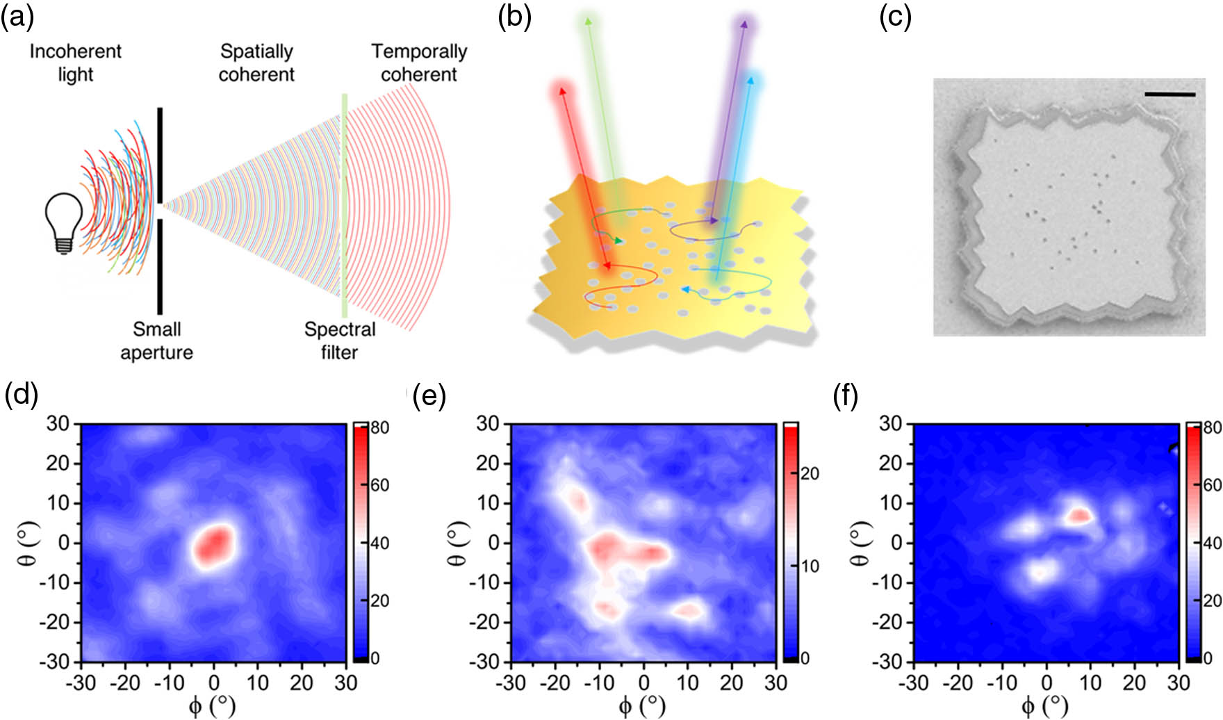
Incoherent light sources, including thermal sources and light emitting diodes (LED), are usually employed to prevent coherent artifacts and obtain high-quality speckle-free images, but they suffer from low intensity ( $\sim 50 lm/W$ ) [5]. Their spatial coherence [6,7] is commonly controlled by spatial filtering [see sketch in Fig. 1(a)] with a pinhole or a microscope objective that selects the light from a portion of the emission area, artificially inducing partial coherence, at the price of an additional reduction of the power output [4].

Figure 1.(a) Coherence property of a light source that from being totally incoherent can be made spatially coherent by spatial filtering with a small aperture, and temporally coherent with a spectral filter. (b) Random distribution of scattering centers in random THz QCLs (gray holes) that provide optical feedback (colored arrows) and act as light out-couplers for multimode emission. (c) Scanning electron microscope image of a random THz QCL showing the hole pattern and irregular edges made to suppress Fabry–Perot modes. Scale bar corresponds to 50 μm. (d)–(f) Far-field intensity patterns of three random THz QCLs named (d) A, (e) B, and (f) C having different $r / a_{s}$ ratios, measured at 80% of their total peak power.

Alternative approaches to induce partial spatial coherence rely on the use of high-spatial-coherence laser sources combined with a time varying optical diffuser [8,9]. Once implemented in an imaging system, this solution, however, requires motorized control of the diffuser motion and a much longer acquisition time, due to the need to generate a set of independent speckle patterns [9].

Sign up for Photonics Research TOC. Get the latest issue of Photonics Research delivered right to you！Sign up now

A valuable approach to tune the spatial coherence while preserving the power output relies on the use of a peculiar class of lasers: random lasers [10 –12].

Random lasers are unconventional lasers since they do not require a resonant cavity to provide optical feedback for enhancing the stimulated emission [13]. They rely on multiple scattering processes generated in a highly disordered gain medium [14,15] that localize photons and supply the feedback for the lasing oscillation [Fig. 1(b)]. The feedback can be non-resonant [16] (incoherent) or resonant (coherent), depending on how the scattering occurs, i.e., in a weak or strong regime, along open or closed trajectories in the random medium [15].

As a distinctive characteristic, random lasers exhibit coherent emission, a property independent of the degree of localization of the emitted optical modes and of the amount of “coherent” feedback.

The large interaction length associated with the random walk that photons undergo in the active medium results in an emission characterized by high temporal coherence [10 –12]. On the other hand, a large number of modes with uncorrelated phases lase simultaneously and combine to produce an emission with low spatial coherence [2,17 –19]. While conventional laser sources have high spatial coherence [1], due to the use of resonant cavities with a limited number of spatial modes that produce well-defined wavefronts, the opposite occurs in a random laser, which, by definition, is based on the emission of randomly distributed modes with distinctly structured wavefronts.

Different disordered media have been proposed so far to support random lasing, including laser dye particles [20,21], glasses [22,23], and powders [24,25]. In the mid-infrared [26,27] and terahertz (THz) [28 –30] frequency ranges, random lasing with large quantum efficiencies has been achieved by exploiting electrically pumped quantum cascade lasers (QCLs), in which coherent feedback is provided by surface disordered photonic structures, implemented on bi-dimensional resonators of dissimilar geometries [28 –31].

At THz frequencies, of wide interest for the undisguised potential for imaging and tomography, random lasing has been demonstrated only in QCLs. They have been engineered with a disordered distribution of air pillars [12,29], dielectric pillars [30], or a combination of semiconductor and metal pillars [31] extended through the active region or only through the highly doped semiconducting top cladding [8], the latter resulting in a stable continuous wave (CW) random laser emission over an optical bandwidth of 430 GHz [28]. In these architectures, the air holes act simultaneously as scattering centers, providing the required optical feedback, and as out-couplers, providing the extraction feedback, for vertical light out-coupling [Fig. 1(b)].

Random THz QCLs prove also to be sensitive to optical feedback and have been employed for near-field imaging applications in a detectorless configuration, exploiting the intracavity reinjection of the laser field via self-mixing interferometry [32], or in the far field, in combination with a sensitive detector.

This achievement opens key application perspectives. THz imaging technologies can indeed strongly benefit from the development of high-radiance THz sources with tunable coherence properties. The use of THz radiation to spatially resolve the properties of materials can provide complementary information [33] to microwaves and infrared, visible, ultraviolet, or X-ray imaging, offering a number of advantages including: higher spatial resolution than microwaves, longer penetration depth for many plastics and composites compared to infrared, high contrast to materials with large static dipole content (e.g., water) or large electrical conductivity (e.g., metals), and high chemical sensitivity based on spectroscopic fingerprints related to THz vibrational modes.

Assessing experimentally the spatial coherence of a random THz laser is not only of fundamental interest, but since this characteristic is likely to be quite different for random lasers than for conventional THz lasers, it also could lead to a set of applications in which random lasers could outperform conventional lasers. As an example, optical coherence tomography [33,34] and laser ranging [35,36] are limited by spatial cross talk and speckle and could benefit from the development of an intense, spatially incoherent light source.

Here we experimentally measure the spatial coherence of a set of electrically pumped THz QCL multimode random lasers sharing a different disordered arrangement of scatterers, performing a Young’s double-slit experiment, and we provide a concrete demonstration of their imaging capabilities in comparison with Fabry–Perot (FP) THz QCLs exploiting the same active region design.

2. RESULTS

We fabricate three sets of random THz QCLs following the architecture described in Refs. [28,32,37]; the same QCL active medium is sandwiched between two highly doped semiconductor metallic cladding layers and processed in an Au–Au double-metal waveguide. Holes of radius $r$ are then patterned on the top resonator metal surface and etched through the highly doped semiconductor top cladding [Fig. 1(c)]. Homogenous current injection is ensured by the symmetrical positioning of four bonding wires at the vertices of the squared metal top surface. Extensive details on the fabrication can be found in Ref. [28]. The three lasers, labeled as samples A, B, and C, share a very low filling fraction ( $FF = 2 %$ ) and differ in the hole radius r, which is 3 μm in samples A and C and 5 μm in sample B, and in average side $L$ , which is 325 μm for samples A and B and 200 μm for sample C. The three lasers have a distinct random arrangement of holes [see Appendix A, Figs. 6(a)–6(c)], generated with a software built on MATLAB, corresponding to defined average inter-site distance $a_{s} = L / \sqrt N$ , where $N$ is the number of holes. This defines a geometrical filling factor $r / a_{s}$ that varies from 8.5% (sample A, $N = 90$ ) to 12% (sample B, $N = 54$ ) and 6.5% (sample C, $N = 19$ ). The spatial autocorrelation function of the hole arrangement is very similar for samples A and C, while it decays slower with the distance in the case of sample B [see Appendix A, Fig. 6(d)] indicating a slightly higher short-range disorder.

To suppress spurious FP or whispering-gallery modes that can form within the double-metal waveguide, the mesa border of the photonic structure is surrounded by an absorbing chromium layer with an irregular shape featuring protrusions of $\approx 25 μm$ [Fig. 1(c)], of comparable size with the wavelengths of the expected lasing modes in the active core, i.e., $\approx 35 μm$ (at 3 THz).

The dissimilar spatial distribution of scatterers results in a specific polarization of the emitted modes, power extraction, and emitted spectrum [37]. The light-current and voltage-current characteristics (L-I-V), spectra, and the polarization plots of the three lasers are reported in Appendix B [Figs. 7(a), 7(b)–7(d), and 8, respectively). The emission spectra of samples A and B are reported also in Ref. [37], while that of sample C is also discussed in Ref. [32]. Sample A displays a rich spectrum with up to 11 random optical modes at peak power [37], unpolarized emission, and larger power output compared to samples B and C [see Appendix B, Fig. 7(a)]. Light polarization can be exploited for imaging specimens with polarization-dependent optical properties.

The far-field profiles of samples A–C at a driving current corresponding to 80% of the total maximum power are acquired with a pyroelectric detector placed at 36 mm from the laser source with a 1 mm entrance slit, 0.5 mm steps, and 30 ms integration time; see Figs. 1(d)–1(f). The intensity distribution reflects the interference pattern resulting from the dipole (scatterers) distribution on the top surface varying from a low-divergence, well-concentrated lobe (10° total divergence) in sample A, to disordered intensity distributions covering a broader surface (35° divergence in sample B; 20° divergence in sample C).

A. Spatial Coherence

We characterize the spatial coherence of the three random THz QCLs by performing a modified Young’s double-slit experiment [38], following the scheme sketched in Fig. 2(a). The light emitted by the random THz QCL sources is diffracted by two small apertures located at a distance $z_{s}$ , and interferes giving rise to the intensity patterns reported in Figs. 2(b) and 2(c) (right side), acquired for two orthogonal orientations of the double-slit interferometer [left side, Figs. 2(b) and 2(c)]. The interferometer is located at $z_{s} = 36 mm$ from the source and consists of two rectangular apertures of width $a = 1 mm$ and with center–center separation $d = 3 mm$ . The slits can be here considered one-dimensional since their length $L_{s} = 40 mm$ exceeds the laser spot diameter at $z = z_{s}$ . The experiment focuses on the measurement of the Fraunhofer diffraction pattern [39], a condition fulfilled by placing the interferometer at a distance $z > a$ , $d$ and larger than the size of the scanned area. A polymethylpentene (TPX) lens (with focal length $f = 200 mm$ ) is placed after the mask at 2 mm distance, to concentrate the intensity pattern on $a \sim 50 mm$ region and compensate for the small throughput of the interferometer. We acquire rectangular maps of size $15 mm \times 90 mm$ , oriented with the longer side parallel to the slits’ axes, along which the intensity modulation is expected. The pattern is recorded at a distance $z = f$ from the lens by a pyroelectric detector that scans on the view plane along $x y$ with 0.4 mm steps. To increase the spatial resolution of the pyroelectric detector, which has a circular $7 {mm}^{2}$ sensitive area, we use a 1 mm entrance slit.

Figure 2.(a) Schematics of the experimental setup for modified Young’s double-slit experiment. (b), (c) From top to bottom, interference patterns of samples A, B, and C acquired by placing the slits (b) parallel to the optical table or (c) orthogonal to the optical table. The noise levels are 7, 6, and $2 \times 10^{- 1}$ for lasers A, B, and C, respectively, estimated as average intensity over a $10 \times 10 pixels$ dark region. (d), (e) Average cross-section intensity distribution evaluated from maps in (b) and in (c) considering two pixels (colored curves) or 30 pixels (black solid line). (f) Spatial coherence value evaluated from the visibility of the fringes in (d) and (e) obtained with a horizontal (H, right panel) or vertical (V, left panel) orientation of the slits, as a function of the vertical coordinate Y (colored open dots) and compared to the values obtained in an FP THz QCL (dashed black line).

According to the Huygens–Fresnel principle, the interference pattern results from the superposition of contributions from point sources distributed along the two slits that, in the case of partially coherent sources, form a collection of incoherent sources that emit light independently.

From the maps in Figs. 2(b) and 2(c), we extract the averaged cross-section intensity profiles reported in Figs. 2(d) and 2(e) (solid black line). Interestingly, the fringes’ visibility largely varies along the slit direction, as a consequence of the inhomogeneous far-field pattern illuminating the interferometer given by the superposition of various lasing modes with different spatial profiles [37]. To quantify the variation along the direction orthogonal to the slits’ axes, we averaged the maps vertically over two pixels (0.8 mm scan range) and compared the fringes along 15 mm scans in the case of horizontally and vertically oriented slits [see colored lines in Figs. 2(d) and 2(e)]. The distance between the fringes’ maximum and minimum, and accordingly the spatial periodicity of the fringes, depends on the spectral content of the diffracted light [38] and varies in the range of 1.2–4.2 mm. The small change in spatial periodicity ( $< 2 mm$ ), expected when the frequency of the optical mode changes in the range of 2.9–3.4 THz, prevents tracing the spatial variation of the far-field spectrum from the variation of the spatial periodicity of the fringes [38]. From the visibility of the interference fringes, we quantify the spatial coherence of the three sources defined as $μ = (I_{\max} - I_{\min}) / (I_{\max} + I_{\min})$ , where $I_{\max}$ is the central highest peak value, and $I_{\min}$ is the neighboring valley value. The spatial coherence $μ$ can range from zero to one, where zero identifies a completely spatially incoherent source and one a fully spatially coherent light. The spatial coherence values in Fig. 2(f), retrieved from the fringes determined by the horizontal (vertical) slits, vary around the values: 0.35 (0.36) for sample A, 0.13 (0.32) for sample B, and 0.22 (0.30) for sample C; see Fig. 2(f), solid lines. Sample A, which exhibits unpolarized emission, produces fringes with the highest visibility and spatial coherence values, similar for the two slits’ orientations. On the contrary, for samples B and C, the retrieved spatial coherence consistently increases when the slits are oriented horizontally and their axes are aligned with the field polarization. We note that the lowest spatial coherence is shown by sample B, having the largest size, largest correlation radius (see Appendix A), and largest beam divergence. Comparing samples A and C, which have similar correlation radii, we observe that the laser with higher divergence (sample C) shows lower spatial coherence. The variation along Y of the spatial coherence in Fig. 2(f), as quantified by the standard deviation, for horizontal (vertical) slits is 0.06 (0.08) for sample A, 0.07 (0.09) for sample B, and 0.06 (0.05) for sample C. We note that if we consider $0 < Y < 12 mm$ , the fringes of sample B, measured with vertically oriented slits, display the smallest spatial variation equal to 0.02. These spatial coherence values can be compared to the values 0.02 of the LED ( $λ = 635 nm$ ), 0.49 of the microLED, and 0.67 of the super luminescent LED ( $λ = 662 nm$ ) recently characterized by a similar double-slit experiment [4]. Interestingly, an FP THz QCL, based on the same active region design but exploiting a resonant cavity reveals, as expected, a much higher spatial coherence with $μ = 0.82$ (see Appendix D, Fig. 9), confirming that the random lasing process significantly reduces the spatial coherence.

The performed experiment reveals that our random THz QCL sources are not completely incoherent. Such a result is not only not surprising, considering the reduced size of the emitting surface (comparable to $λ$ ) and the low divergence, but it offers peculiar advantages for THz imaging: partial coherence is indeed desirable for reducing artifacts due to interference, and speckles, with respect to high coherence sources, and permits the application for holographic imaging by preserving a phase relation between different points of the image. Consequently, random THz QCLs can offer concrete benefits for imaging applications.

B. Imaging Sharpness and Speckles

To analyze the relation between spatial coherence and imaging capability of our random THz QCLs, we built a confocal microscope working in transmission geometry, as sketched in Fig. 3(a). The light emitted by the random THz QCL is collimated with a 90° off-axis parabolic mirror (OAP) with 50 mm focal length and focused on the sample over a spot of $\sim 500 μm$ by a second OAP with 50 mm focal length. The lasers are driven in pulsed mode at 100 kHz with 10% duty cycle (using Avtech AVR series, medium to high voltage general purpose pulse generators) at the same peak currents used in Figs. 1 and 2, and we impose a modulation at 33 Hz to the laser driver to match the electronic bandwidth of the thermal detector. The light transmitted by the sample is collected with an OAP of 50 mm focal length and focused on a pyroelectric detector by means of a TPX lens with 50 mm focal length. The signal of the pyroelectric detector is recorded at 33 Hz with a lock-in amplifier (Zurich Instrument UHLI). By raster scanning the sample in the focal plane, we spatially resolve its THz transmission.

Figure 3.(a) Experimental setup for confocal imaging based on random THz QCLs. (b) Photo of the maple seed we used to test our imaging setup; scale bar corresponds to 5 mm. (c) Transmission images of the sample acquired with sample A (panels on the left) and sample B (panels on the right) with open (top panels) and closed pinholes (bottom panels). The brightness of all the images is normalized for better comparison. Histogram reporting the distribution of pixel intensity around the average value $⟨ I ⟩$ calculated for the images in (c) with open (gray) and closed pinholes (red) for samples (d) A and (e) B.

We image the maple seed in Fig. 3(b), which is mapped with steps of 250 μm integrating 30 ms per pixel. The images obtained with samples A and B are reported in Fig. 3(c), while analogous images taken with sample C using a smaller seed are shown in the Appendix E [Figs. 12(a) and 12(b)]. Our imaging system is capable of resolving the seed shape and reveals the contrast of leaf veins to THz radiation due to water absorption. To isolate the effect of spatial coherence on image quality, we compare the images taken with the bare random laser source with the ones obtained by inserting a pinhole of 1 mm diameter to increase the spatial coherence by spatial filtering [see Fig. 3(c)]. An attenuator is placed before the pyroelectric detector to maintain the same average counts in the two configurations. We can observe a drastic change in the THz images, which is partially due to an increase in image sharpness with the closed pinhole, and partially to a change in the speckle pattern.

To quantify the differences in speckles, we analyze the distribution of pixel intensity around the mean intensity value $⟨ I ⟩$ averaged on a $1 cm \times 3 cm$ area; see Figs. 3(d) and 3(e). Analogous data for sample C are reported in Appendix E [Fig. 12(c)]. We define speckle contrast $C$ as the standard deviation $σ$ of the intensity fluctuation divided by the mean intensity value $⟨ I ⟩$ in the area of interest, as in Ref. [4]. A speckle contrast of one indicates totally spatially coherent light, while a speckle contrast of zero corresponds to spatially incoherent light. The images in Fig. 3, taken with sample A, exhibit a speckle contrast of 0.38 without the pinhole and 0.59 with the pinhole; for sample B, we have 0.49 without the pinhole and 0.59 with the pinhole. Thus, the speckle contrast retrieved with the closed pinhole in both cases is the same, indicating that the higher spatial coherence can be ascribed to the pinhole itself.

Interestingly, the fabricated random THz QCLs can operate at up to 55 K without a significant reduction in emitted power [28]. Accordingly, we use a Stirling cryocooler to refrigerate the laser driven in pulsed mode, maintaining a fixed temperature of 40 K.

To discard the possible impact of the improved spatial resolution in pixel intensity distribution, we repeat the same experiment by placing in the object plane a scattering film (see Fig. 4) consisting of a lint-free paper tissue. The intensity distribution measured with laser C is Gaussian-like in both cases, while the speckle contrast varies from 0.27 to 0.34 when a pinhole is employed.

Figure 4.(a) Transmission images of a $2 cm \times 2 cm$ ( $100 \times 100 pixels$ ) lint-free paper tissue measured with sample C with (a) open and (b) closed pinholes. (c) Histogram reporting the distribution of pixel intensity around the average value $⟨ I ⟩$ calculated for the images in (a), (b) with open (gray) and closed pinholes (red).

To characterize the resolution of our imaging system, we use a custom-made test chart, inspired by the 1951 US Airforce test chart [Fig. 5(a)]. The chart contains various target shapes of linear dimension ranging from 0.2 to 2 mm, organized in groups of three bars forming minimal Ronchi rulers that provide an assortment of spatial frequency specimens and allow correction for spurious resolution artifacts. The positive target is prepared depositing 7 nm/14 nm of Cr/Au on a ${SiO}_{2} / Si$ wafer with $\sim 80 %$ transmission at 3 THz. For given collimation optics, the spatial resolution of the imaging system depends on the laser divergence, which determines the waist of the collimated beam. The larger the beam radius that reaches the focusing mirror, the smaller the spot size at the object plane and the higher the spatial resolution. Accordingly, the sample with the largest divergence is expected to give the highest spatial resolution.

Figure 5.(a) Resolution test chart made by evaporating 7 nm/40 nm Cr/au on a SiO₂/Si slide. (b), (c) THz transmission images of the test chart acquired with (b) FP laser and (c) sample A. (d) Contrast-to-noise ratio (CNR) evaluated from the analysis of 18 Ronchi rulers in the images acquired with the FP and random lasers, in (b) and (c), respectively. (e) Speckle contrast of the images acquired with sample A as a function of pinhole diameter. (f) Spatial resolution of the images acquired with sample A as a function of pinhole diameter. Images from which the data in (e) and (f) are extracted can be found in Appendix E.

Figures 5(b) and 5(c) show the images obtained in transmission with sample A and with an FP THz QCL sharing an identical active core. Image quality can be compared quantitatively using the contrast-to-noise ratio (CNR), defined [2] as $(⟨ I_{f} ⟩ - ⟨ I_{b} ⟩) / \frac{σ_{f} + σ_{b}}{2}$ , where $⟨ I_{f} ⟩$ is the average intensity within the three bars composing each ruler, $⟨ I_{b} ⟩$ is the average intensity in the surrounding (background), and $σ_{f}$ and $σ_{b}$ are the standard deviation in the bars and in the background, respectively.

When CNR approaches unity, feature contrast is comparable to image noise. We evaluate the CNR considering 18 different Ronchi rulers, each corresponding to a different spatial frequency in the range of $3 − 12 pixels {mm}^{- 1}$ . We can see that despite the image obtained with the FP laser having higher resolution, it has a lower CNR than the random laser, due to the higher spatial coherence. In Fig. 5(e), we report the variation of the speckle contrast measured with the random laser (sample A) considering the $2 mm \times 2 mm$ ( $20 \times 20 pixels$ ) squared feature of the test chart, as a function of the diameter of the pinhole inserted in the path. By closing the pinhole, the speckle contrast increases as a consequence of the increased spatial coherence. By reducing the pinhole diameter, we also observe an improvement in the resolution, from 0.62 up to 0.54 mm, obtained with a 1 mm diameter pinhole.

3. DISCUSSION

Compared to thermal sources, a random laser can be designed to emit light with low spatial coherence to eliminate coherent artifacts while maintaining a low divergence and a high power per mode. At the driving currents used in the experiments, corresponding to 80% of the total maximum power, including contribution from all emitted modes, sample A has 70% of the power ( $\sim 7.8 mW$ ) concentrated in one mode at 3.1 THz, while the rest is distributed on six additional modes with a minimum power per mode of 0.2 mW. In sample B, there are four modes in total, but 90% of the power ( $\sim 3.6 mW$ ) is concentrated in the mode at 3.1 THz, and the minimum power per mode is lower (80 μW). Finally, in sample C, 45% of the power ( $\sim 2.7 mW$ ) is concentrated on the mode at 3.4 THz, while the rest is almost equally distributed among four additional modes, such that the minimum power per mode is 1 mW. We can compare these sources to other partially coherent sources in terms of number of photons per coherence volume or photon degeneracy. It is worth mentioning that the photon degeneracy parameter $d$ is directly proportional to the spectral radiance, a radiometric measure of the amount of radiation through a unit area and into a unit solid angle within a unit frequency bandwidth. The low spatial coherence of our random THz QCLs is particularly useful for imaging in scattering environments, which are common in biological imaging or imaging through atmospheric turbulence. Scattered photons can indeed interfere if they are spatially coherent, corrupting the image beyond shape recognition. Accordingly, a coherent source, that in normal conditions would allow for resolving objects with higher spatial resolution than a partially coherent source, can become useless in a scattering environment due to photon cross talk.

4. CONCLUSION

We assess experimentally the spatial coherence of a set of multimode random THz QCLs having dissimilar photonic patterns, performing a Young’s double-slit experiment. A partial spatial coherence between 0.16 and 0.34, depending on the specific disorder, is found, significantly lower than that (0.82) retrieved on the corresponding FP THz QCL. The partial coherence of random THz QCLs, combined with laser-level power and low divergence, leads to superior performances in terms of speckles and spatial cross talk in imaging applications across the far infrared. We observe that the spatial coherence is minimized by increasing the correlation radius of the random patterns of holes, which also results in an increased beam divergence. Accordingly, our study suggests that photonic random patterns with larger correlation radii allow reducing imaging coherent artifacts. The achieved results open groundbreaking perspectives for THz applications in which the latter can provide major benefits such as biomedical inspection, cancer diagnostics, pharmacological tomography, food control, process and quality inspection, securing and postal scanning, cultural heritage, and sophisticated nanoscopy experiments in the far infrared aimed at mapping light–matter interaction modes and phenomena at the nanoscale. As a final perspective, random THz QCLs can be nowadays engineered to work at higher temperatures, up to $\sim 250 K$ [40], in a thermoelectrically cooled environment, by properly optimizing the active region design, as recently demonstrated for FP THz QCLs [40,41], and carefully engineering the device thermal management [42]. This can allow extending the described application potential to portable and compact systems.

Acknowledgment

Acknowledgment. We thank Dr. Elisa Riccardi for the custom-made test chart used in the imaging experiments.

APPENDIX A: RANDOM PATTERNS

r = 3 μm

Figure 6.Random pattern of surface holes in samples (a) A, (b) B, and (c) C, and (d) spatial autocorrelation function in the three cases evaluated as in Refs. [28,37]. The patterns and autocorrelation function for samples A and B are also reported in Ref. [37].

APPENDIX B: VOLTAGE–CURRENT DENSITY AND LIGHT–CURRENT DENSITY CHARACTERISTICS

J_{th, A} \sim 440 A / {cm}^{2}

Figure 7.(a) Voltage–current density and light–current density characteristics of samples A, B, and C measured driving the devices in pulsed mode with a pulse width of 10 μs (duty cycle 10%) at a heat sink temperature of 15 K. The black star symbols indicate the operating currents at which the double-slit experiments are performed. (b)–(d) FTIR spectra of samples (b) A, (c) B, and (d) C, measured at the current densities indicated by black star symbols in (a).

Figures 7 (b)- 7 (d) show the Fourier transform infrared (FTIR) emission spectra of samples A, B, and C at the current density values marked in Fig. 7 (a).

APPENDIX C: POLARIZATION

7 {mm}^{2}

Figure 8.Polar plot of laser intensity as a function of polarization angle $α$ for samples (a) A, (b) B, and (c) C measured filtering the emission with a linear polarizer placed just before the pyroelectric detector.

APPENDIX D: FRINGES AND SPATIAL COHERENCE OF A FABRY–PEROT THz QUANTUM CASCADE LASER

20 mm \times 85 mm

μ = 0.82

Figure 9.Interference fringes of an FP THz QCL performing a modified Young’s double-slit experiment. (a) Map of the $20 mm \times 85 mm$ region scanned with the pyroelectric detector; (b) cross-section average intensity of the map in (a) showing interference fringes.

Figure 10.(a) Continuous wave current-voltage-power characteristics of an FP THz QCL. (b) Normalized Fourier transform infrared (FTIR) emission spectrum of the FP THz QCL, measured at $J = 365 {A / cm}^{2}$ .

Figure 11.Far-field intensity pattern of FP THz QCL, measured at $I = 657 mA$ ( $J = 365 {A / cm}^{2}$ ).

APPENDIX E: CONFOCAL MICROSCOPY IMAGING WITH SAMPLE C

C = 0.62

Figure 12.THz transmission image of a maple seed obtained using sample C driven at $J_{C} = 549 A / {cm}^{2}$ (a) without inserting the pinhole and (b) with the pinhole. Images are normalized for comparison. (c) Distribution of pixel intensities around the average value $⟨ I ⟩$ of the image with open pinhole (gray histogram) from (a), and with closed pinhole (red histogram) from (b).

APPENDIX F: EFFECT OF SPATIAL FILTERING ON IMAGE QUALITY

3.5 mm \times 3.5 mm

Figure 13.Comparison of THz images of a test chart acquired with sample A, as it is and after filtering its emission with a pinhole of diameters ranging from 3 mm to 1 mm, as indicated in the image title.

Figure 14.Linecuts of maps in Fig. 13 at the edge of the open squared feature of the test chart. Data are reported as colored dots; fits with the edge function described in the text to evaluate the spatial resolution of the images are shown as solid colored lines.

References

[1] L. Mandel, E. Wolf. Optical Coherence and Quantum Optics(1995).

[2] B. Redding, M. A. Choma, H. Cao. Speckle-free laser imaging using random laser illumination. Nat. Photonics, 6, 355-359(2012).

[3] https://www.sciencedirect.com/topics/physics-and-astronomy/holography. https://www.sciencedirect.com/topics/physics-and-astronomy/holography

[4] Y. Deng, D. Chu. Coherence properties of different light sources and their effect on the image sharpness and speckle of holographic displays. Sci. Rep., 7, 5893(2017).

[5] https://web.archive.org/web/20090505080533/http://www1.eere.energy.gov/buildings/ssl/comparing.html. https://web.archive.org/web/20090505080533/http://www1.eere.energy.gov/buildings/ssl/comparing.html

[6] D. S. Mehta, K. Saxena, S. K. Dubey, C. Shakher. Coherence characteristics of light-emitting diodes. J. Lumin., 130, 96-102(2010).

[7] F. J. Duarte. Coherent electrically excited organic semiconductors: visibility of interferograms and emission linewidth. Opt. Lett., 32, 412-414(2007).

[8] T. M. Rohith, H. Farrokhi, J. Boonruangkan, Y. J. Kim. Spatial coherence reduction for speckle free imaging using electroactive rotational optical diffusers. Conference on Lasers and Electro-Optics Pacific Rim (CLEO-PR), 1-2(2017).

[9] H. Zhang, K. Wiklund, M. Andersson, T. Stangner, T. Dahlberg. Step-by-step guide to reduce spatial coherence of laser light using a rotating ground glass diffuser. Appl. Opt., 56, 5427-5435(2017).

[10] H. Cao, J. Y. Xu, D. Z. Zhang, S.-H. Chang, S. T. Ho, E. W. Seelig, X. Liu, R. P. H. Chang. Spatial confinement of laser light in active random media. Phys. Rev. Lett., 84, 5584-5587(2000).

[11] H. Cao. Random lasers: development, features and applications. Opt. Photon. News, 16, 24-29(2005).

[12] D. S. Wiersma. The physics and applications of random lasers. Nat. Phys., 4, 359-367(2008).

[13] R. Sapienza. Determining random lasing action. Nat. Rev. Phys., 1, 690-695(2019).

[14] B. Wunsch, T. Stauber, F. Sols, F. Guinea. Dynamical polarization of graphene at finite doping. New J. Phys., 8, 318(2006).

[15] H. Cao, J. Y. Xu, Y. Ling, A. L. Burin. Lasing in disordered media. Quantum Electronics and Laser Science Conference, 1(2002).

[16] D. Grigsby, G. Zhu, J. Novak, M. Bahoura, M. A. Noginov. Optimization of the transport mean free path and the absorption length in random lasers with non-resonant feedback. Opt. Express, 13, 8829-8836(2005).

[17] B. Redding, H. Cao, M. A. Choma. Spatial coherence of random laser emission. Opt. Lett., 36, 3404-3406(2011).

[18] B. H. Hokr, M. S. Schmidt, J. N. Bixler, P. N. Dyer, G. D. Noojin, B. Redding, R. J. Thomas, B. A. Rockwell, H. Cao, V. V. Yakovlev, M. O. Scully. A narrow-band speckle-free light source via random Raman lasing. J. Mod. Opt., 63, 46-49(2015).

[19] H. Cao, Y. Ling, J. Y. Xu, A. L. Burin. Probing localized states with spectrally resolved speckle techniques. Phys. Rev. E, 66, 025601(2002).

[20] S. García-Revilla, J. Fernández, M. Barredo-Zuriarrain, E. Pecoraro, M. A. Arriandiaga, I. Iparraguirre, J. Azkargorta, R. Balda. Coherence characteristics of random lasing in a dye doped hybrid powder. J. Lumin., 169, 472-477(2016).

[21] N. M. Lawandy, R. M. Balachandran, A. S. L. Gomes, E. Sauvain. Laser action in strongly scattering media. Nature, 368, 436-438(1994).

[22] M. Peruzzo, M. Gaio, R. Sapienza. Tuning random lasing in photonic glasses. Opt. Lett., 40, 1611-1614(2015).

[23] X. Meng, K. Fujita, S. Murai, J. Konishi, M. Mano, K. Tanaka. Random lasing in ballistic and diffusive regimes for macroporous silica-based systems with tunable scattering strength. Opt. Express, 18, 12153-12160(2010).

[24] H. Cao, Y. G. Zhao, S. T. Ho, E. W. Seelig, Q. H. Wang, R. P. H. Chang. Random laser action in semiconductor powder. Phys. Rev. Lett., 82, 2278-2281(1999).

[25] A. Migus, C. Gouedard, C. Sauteret, D. Husson, F. Auzel. Generation of spatially incoherent short pulses in laser-pumped neodymium stoichiometric crystals and powders. J. Opt. Soc. Am. B, 10, 2358-2363(1993).

[26] H. K. Liang, B. Meng, G. Z. Liang, Q. J. Wang, Y. Zhang. Electrically pumped mid-infrared random lasers. Adv. Mater., 25, 6859-6863(2013).

[27] G. Liang, Q. J. Wang, Y. Zeng. Random lasers in the mid-infrared and terahertz regimes. Laser Science 2017, LTh4F.1(2017).

[28] S. Biasco, H. E. Beere, D. A. Ritchie, L. Li, A. G. Davies, E. H. Linfield, M. S. Vitiello. Frequency-tunable continuous-wave random lasers at terahertz frequencies. Light Sci. Appl., 8, 43(2019).

[29] S. Schönhuber, M. Brandstetter, T. Hisch, C. Deutsch, M. Krall, H. Detz, A. M. Andrews, G. Strasser, S. Rotter, K. Unterrainer. Random lasers for broadband directional emission. Optica, 3, 1035-1038(2016).

[30] Y. Zeng, G. Liang, H. Liang, S. Mansha, B. Meng, T. Liu, X. Hu, J. Tao, L. Li, A. Davies, E. Linfield, Y. Zhang, Y. Chong, Q. Wang. Designer multimode localized random lasing in amorphous lattices at terahertz frequencies. ACS Photon., 3, 2453-2460(2016).

[31] Y. Zeng, G. Liang, B. Qiang, K. Wu, J. Tao, X. Hu, L. Li, A. G. Davies, E. H. Linfield, H. K. Liang, Y. Zhang, Y. Chong, Q. J. Wang. Two-dimensional multimode terahertz random lasing with metal pillars. ACS Photon., 5, 2928-2935(2018).

[32] K. S. Reichel, E. A. A. Pogna, S. Biasco, L. Viti, A. Di Gaspare, H. E. Beere, D. A. Ritchie, M. S. Vitiello. Self-mixing interferometry and near-field nanoscopy in quantum cascade random lasers at terahertz frequencies. Nanophotonics, 10, 1495-1503(2021).

[33] D. M. Mittleman. Twenty years of terahertz imaging [Invited]. Opt. Express, 26, 9417-9431(2018).

[34] H. Nishii, T. Nagatsuma, T. Ikeo. Terahertz imaging based on optical coherence tomography [Invited]. Photon. Res., 2, B64-B69(2014).

[35] E. Baumann, J.-D. Deschênes, F. R. Giorgetta, W. C. Swann, I. Coddington, N. R. Newbury. Speckle phase noise in coherent laser ranging: fundamental precision limitations. Opt. Lett., 39, 4776-4779(2014).

[36] B. Redman, R. Chellappa, S. Der. Simulation of error in optical radar range measurements. Appl. Opt., 36, 6869-6874(1997).

[37] A. Di Gaspare, M. S. Vitiello. Polarization analysis of random THz lasers. APL Photon., 6, 070805(2021).

[38] B. J. Pearson, N. Ferris, R. Strauss, H. Li, D. P. Jackson. Measurements of slit-width effects in Young’s double-slit experiment for a partially-coherent source. OSA Contin., 1, 755-763(2018).

[39] M. Born, E. Wolf. Principles of Optics: Electromagnetic Theory of Propagation, Interference and Diffraction of Light(1999).

[40] A. Khalatpour, A. K. Paulsen, C. Deimert, Z. R. Wasilewski, Q. Hu. High-power portable terahertz laser systems. Nat. Photonics, 15, 16-20(2021).

[41] L. Bosco, M. Franckié, G. Scalari, M. Beck, A. Wacker, J. Faist. Thermoelectrically cooled THz quantum cascade laser operating up to 210 K. Appl. Phys. Lett., 115, 010601(2019).

[42] M. S. Vitiello, G. Scamarcio, V. Spagnolo, J. Alton, S. Barbieri, C. Worrall, H. E. Beere, D. A. Ritchie, C. Sirtori. Thermal properties of THz quantum cascade lasers based on different optical waveguide configurations. Appl. Phys. Lett., 89, 021111(2006).