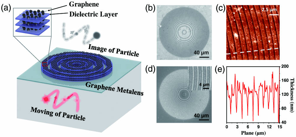
Fig. 1. Design of the particle tracking system with a graphene metalens. (a) Schematic of the lab-on-a-chip particle tracking system with an integrated graphene metalens; inset, structure of graphene metamaterial; (b) reflective optical microscopic image of a fabricated graphene metalens; (c) atomic force microscope (AFM) image of a region of the fabricated graphene metalens; (d) SEM image of the full view and a region of the fabricated graphene metalens; (e) measured cross-sectional thickness distributions along the white dashed line in (c). Scale bars in (b) and (c) are 40 μm. Scale bar in (c) is 2.5 μm. Scale bar in the inset of (d) is 4 μm.

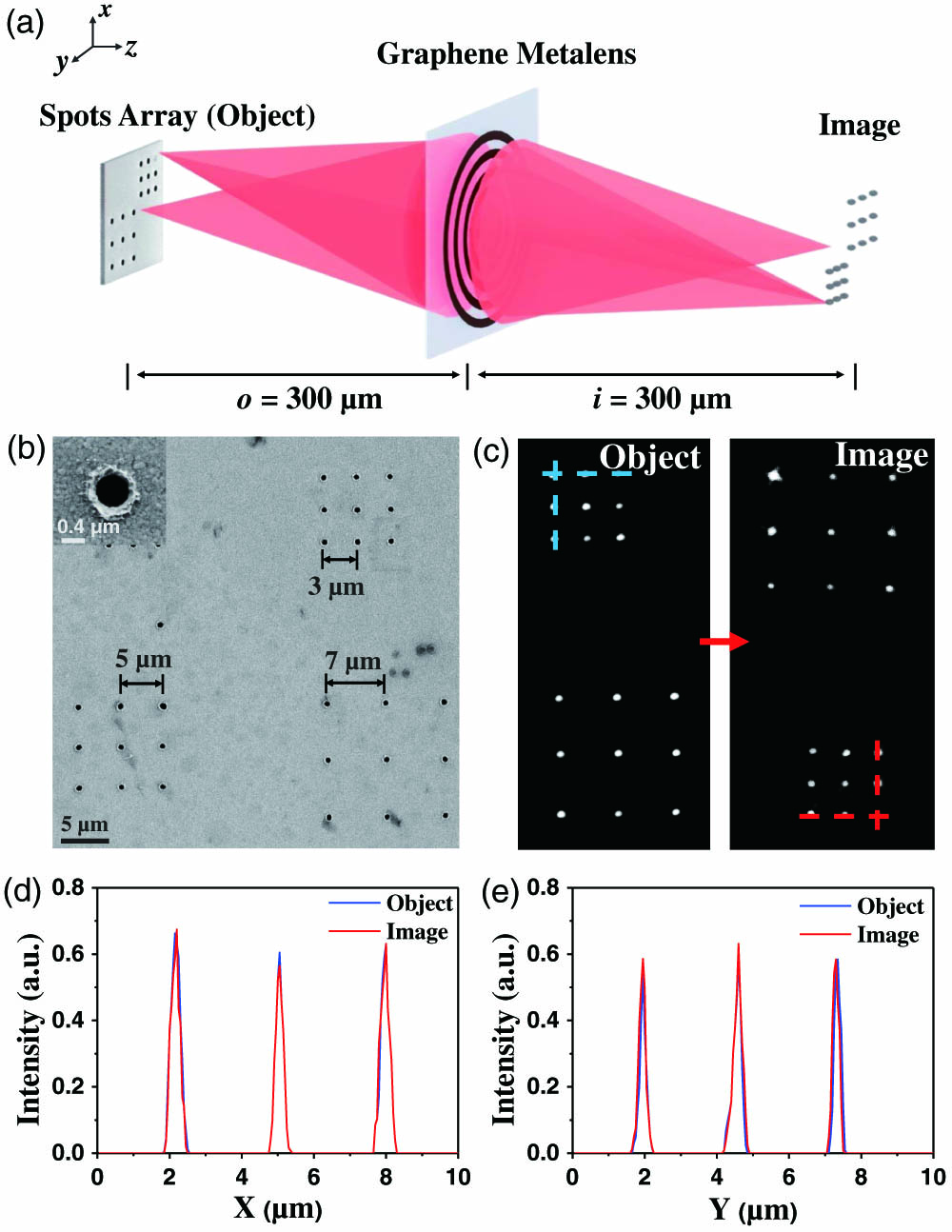
Fig. 2. Imaging performance of the graphene metalens. (a) Schematic of imaging experiment of the spot array object imaged by the graphene metalens. (b) SEM image of the spot array object; (c) optical image of the object and image from the graphene metalens; cross-sectional intensity distribution along the (d) horizontal lines and (e) vertical lines of the spots array from the sample and image. Scale bars in (b) and (c) are 5 μm. Scale bar in the inset of (b) is 0.4 μm.

Fig. 3. Imaging an object moving along the axial direction of the graphene metalens. (a) Schematic for measuring the object and image distances from the lens on the z-axis; (b) measured intensity distribution in the x−z plane with different object distances from 250 to 350 μm; the white dashed line marks the focal plane of the lens where z=300  μm. (c) Calculated and experimentally measured image distance distributions as a function of the object distance.

Fig. 4. Particle tracking analysis using the graphene metalens. (a) SEM image of the fabricated object for PNT demonstration; (b) optical microscopic image of the object; (c) image of the object from the graphene metalens (see Visualization 1); (d) trajectories of three different featured particles as a function of the number of video frames; (e), (f) lateral positions of the object and the image along the x and y directions in different video frames. The frame rate is 15 fps. The scale bars in (a)–(c) are 4 μm.

Fig. 5. (a) Intensity distribution of theoretical results of the graphene metalens with different object distances from 160 to 480 μm; (b) image distance as a function of object distance with RS simulation model and analytical formula.

Fig. 6. (a) Schematic of the focusing characterization of the graphene flat lens; (b) simulated focal intensity distribution along the optical axis; (c) intensity distribution of the 3D focal spot of the graphene flat lens; experimentally measured intensity distributions in the (d) lateral and (e) axial planes; cross-sectional intensity distributions along the white dashed lines in the (f) lateral and (g) axial planes.

Fig. 7. Schematic diagram of the experimental setup used for imaging with the graphene metalens. The laser beam is a supercontinuum laser filtered by a narrowband filter (600 nm with bandwidth of 40 nm). The target was placed at the focal plane of the graphene metalens with the laser illumination. The Mitutoyo objective (100× magnification; NA, 0.8) was used for providing more intensive illumination on the target. A tube lens with focal length of f=150  mm (Thorlabs, TTL150-A) was selectively used to form an image on the CCD camera. The object is mounted on a 3D scanning stage.

Fig. 8. PNT movie frames. The images of the object and image from the graphene lens of the CTAM logo are recorded by the CCD with the number of frames marked in the figure. The pictures of image from the graphene metalens are flipped by 180° for easy comparison (see Visualization 1). The red and yellow dashed lines are used to mark the trajectories of the object and image. The frame rate is 15 fps.