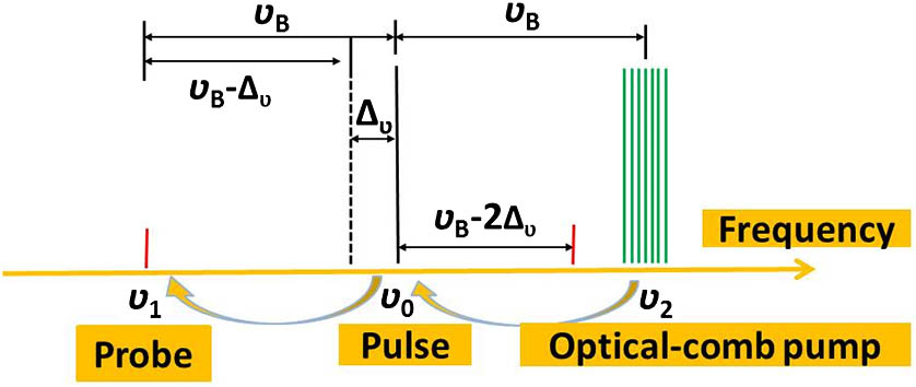
Fig. 1. Principle diagram of DBA-BOTDA with optical-comb pump. The position of the dotted line denotes the frequency of the optical source.

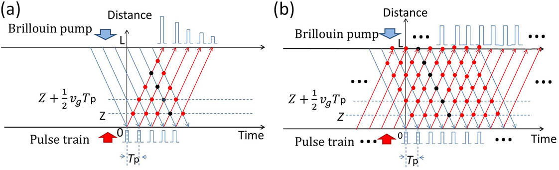
Fig. 2. Schematic diagram of Brillouin pump depletion for coded DBA-BOTDA using (a) non-cyclic and (b) cyclic coding. Tp is the pulse interval. The dots denote the interaction positions. For example, the black dots are the positions where the Brillouin pump has undergone the depletion when the fourth pulse arrives at z.

Fig. 3. Numerical results for pulse gain fluctuation due to pump depletion. (a), (b) Distribution of Brillouin pump. (c), (d) Distribution of coded pulse peak power. (e), (f) Normalized output peak power of coded pulses. (a), (c), (e) are for non-cyclic coding, and (b), (d), (f) are for cyclic coding.

Fig. 4. Experimental setup of coded first-order DBA-BOTDA with optical-comb pump. DFB-LD, distributed feedback laser diode; EOM, electro-optic modulator; EDFA, erbium-doped fiber amplifier; PS, polarization scrambler; VOA, variable optical attenuator; FUT, fiber under test; AOM, acoustic-optic modulator; AWG, arbitrary waveform generator; MWS, micro-wave source; TBPF, tunable bandpass filter; PD, photodetector; DAQ, data acquisition card; OSA, optical spectrum analyzer; OSC, oscilloscope.

Fig. 5. (a) Pulse waveforms after EDFA3. (b) Transmitted pulse waveforms at different pulse peak powers with DBA. (c) 3D BGS near the hot spot at pulse peak power of 15 dBm. (d) BGS at the rising edge of the hot spot. Non-cyclic coding is used.

Fig. 6. (a) Pulse waveforms after EDFA3. (b) Transmitted pulse waveforms at different pulse peak powers with DBA. (c) 3D BGS near the hot spot at pulse peak power of 15 dBm. (d) BGS at the rising edge of the hot spot. Cyclic coding is used.

Fig. 7. (a) Extracted BFS distributions near the hot spot for various pulse peak powers. The squared and dotted lines are for non-cyclic and cyclic coding, respectively. (b) Pulse gain fluctuations for various peak powers. (c), (d) Brillouin responses with different pulse peak powers at 10,845 MHz. (c) and (d) are for non-cyclic and cyclic coding, respectively. The magnified view of the over-shoot is shown in the inset of (a).

Fig. 8. (a) Extracted BFS near the hot spot for various coding lengths. The squared and dotted lines are for non-cyclic and cyclic coding, respectively. (b) Pulse gain fluctuations for various coding lengths. The magnified view of the over-shoot is shown in the inset of (a).

Fig. 9. 3D BGS near the hot spot using (a) linear approximation and (b) log linearization. (c) BGS at 74.131 km (dotted) and 74.190 km (squared) using linear approximation (red) and log linearization (blue). (d) BFS distributions near the hot spot for different pulse peak powers. Cyclic coding is used.

Fig. 10. Distributions of (a) 3D BGS, (b) BFS along FUT, (c) standard deviation, and (d) BFS near the hot spot for various temperatures. In (a) and (b), the temperature of the hot spot is 60°C.