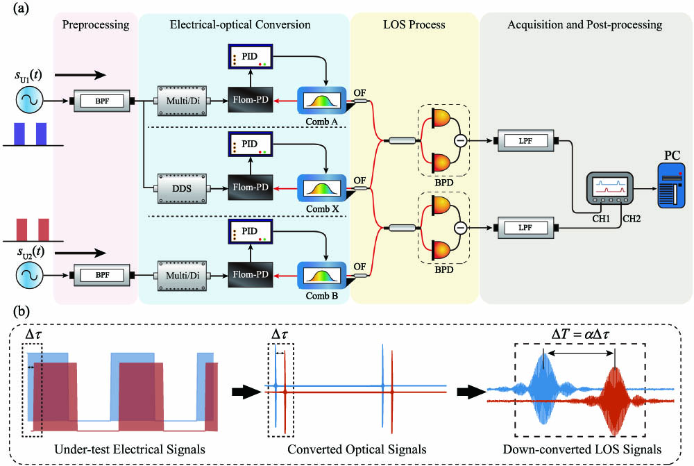
Fig. 1. Schematic of the time interval measurement setup. (a) Time interval measurement setup. The two band-pass filters (BPFs) in the preprocessing part filter a certain harmonic of the under-test pulses, which serve as the combs’ reference after being multiplied, divided, or synthesized. The direct digital synthesizer (DDS) in the electrical-to-optical conversion part generates a sinusoidal wave with a slight frequency difference from its input signal. The repetition frequencies of three combs are phase-locked with the fiber-loop optical-microwave phase detector (FLOM-PD) and the PID. The outputs of combs A and B are sampled through LOS with comb X, and then detected and acquired by balanced photodetectors (BPDs) and an oscilloscope. The low-pass filters (LPFs) are used to isolate the final output. (b) Conversion of the under-test electrical pulses to the measured LOS signals. Through preprocessing and electrical-optical conversion, the signals are converted to two optical-frequency-comb signals, carrying the same time-interval information as the under-test signals. Through the LOS process, the optical signals are down-converted to two LOS signals in terms of the frequency, whose time intervals are amplified α times in comparison with the under-test signals.

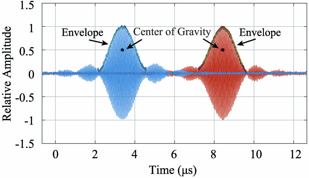
Fig. 2. Processing of the down-converted LOS signal by the envelope calculation and localization (i.e., center finding). The process is achieved by first fitting the signal’s envelope and then calculating its center of gravity.

Fig. 3. Measurement results of system’s precision. (a) Measurement results of the time difference. Black circles represent raw data, while red points represent data processed with the Kalman filter. (b) Measurement precision of the data. Blue crosses indicate the precision of a commercial time-interval counter (Keysight, 53230A). Black circles represent the precision of our work with raw data, while red points represent the precision of our work with processed data.

Fig. 4. Measurement precision (processed data) of the system using 100 MHz sine waves, square waves, and triangular waves. The result shows similar measurement precision for the different waveforms.

Fig. 5. Simulation results of the effect of the relative intensity noise (RIN)-induced time fluctuation. (a) The RIN affects the localization process and brings fitting errors. (b) The time fluctuation is caused by 1.32% RIN, where the sampling rate is set to 500 MHz corresponding to the experimental parameter. (c) The relation of RIN-induced time fluctuation, fCEO-difference, and sampling rate for a fixed RIN level 1.32%. (d) The RIN-induced time fluctuation under the sampling rate of 500 MHz. (e) The RIN-induced time fluctuation under the fCEO-difference of 0 Hz.