
Dongrui Yu, Ziyang Chen, Xuan Yang, Yunlong Xu, Ziyi Jin, Panxue Ma, Yufei Zhang, Song Yu, Bin Luo, Hong Guo. Time interval measurement with linear optical sampling at the femtosecond level[J]. Photonics Research, 2023, 11(12): 2222
- Photonics Research
- Vol. 11, Issue 12, 2222 (2023)
Abstract
1. INTRODUCTION
High-precision time measurement has significant applications in various fields, including remote time synchronization [1–4] and precise navigation systems [5–8]. A prominent example is the research on numerous scientific experiments, where high-precision time measurement can directly limit the experimental performance, such as time-of-flight measurement in high-energy particle physics [9], dark matter detection and measurement of fundamental constants [10–16]. Specifically, high precision is always the ultimate goal of time measurement, and the progression of its technique can help overcome technical bottlenecks in precision measurement in relevant fields and can also bring about a breakthrough in discovering new areas of physics, such as particle physics and cosmology.
Traditional solutions to measure the time interval of electrical signals use electrical means [17–19]. They measured the equivalent voltage proportional to the time interval under test [9,20] or used the digital counting method to directly count the number of clock cycles [9,20–22]. The precision of the former method, with the order of hundred picoseconds (ps), is limited by the poor resolution of digital devices; the latter methods, with the help of the dual mixer time difference measurement technique, can achieve performance better than 0.1 ps [23]. However, such a sub-ps-level time interval measurement cannot satisfy the requirements of state-of-the-art precise implementations, such as gravitational wave detection and femtosecond (fs) level time frequency transfer. To support the rapidly growing precision requirement and the expanding directions of applications, researchers must urgently find a breakthrough approach for precision measurement.
Compared to traditional electrical techniques, optical frequency comb (OFC) based techniques offer a possibility for high-performance time frequency measurement because of their ultrahigh time resolution [24–27]; therefore, this technology enables high-precision time interval measurement. Remarkably, dual OFC based linear optical sampling (LOS) techniques have been extensively studied in many high-precision measurement fields. For example, fs-level remote time synchronization [1,28,29] and nanometer absolute distance measurement [30–33] have been achieved, showing the advantage of using optical means for precision measurement. However, the time interval measurement of electrical signals by optical methods faces numerous technical difficulties, such as the noise introduced by electro-optical conversion, the precision of optical methods, the robustness and complexity of the optical system, and the capability of measuring irregular waveforms, which leads to challenges for high-performance and simple system design.
Sign up for Photonics Research TOC. Get the latest issue of Photonics Research delivered right to you!Sign up now
Here, we demonstrate an optical method for ultrahigh precision time interval measurement that measures two periodic electrical signals with fs-level precision, despite arbitrary waveforms. The electrical pulses under test were locked to the repetition frequencies of two OFCs to transfer the interval information from the electrical to the optical region. By introducing dual-comb LOS technology, we used a third OFC locked to one of the signals being tested to sample the two optical pulses, which in principle overcomes the limitation of electrical means. Because the carrier-envelope offset frequency does not need to be manually stabilized, the complexity of the entire system was significantly reduced. We showed that the precision of the time interval measurement of electrical pulses fell below 3.05 fs after LOS and post-processing. The findings demonstrate the feasibility of the fs-level time interval measurement of electrical pulses and provide support for ultrahigh-precision microwave applications.
2. RESULTS
A. Experimental Setup
A schematic diagram of the time interval measurement system is illustrated in Fig. 1(a). When measuring two input electrical periodic signals with arbitrary waveforms, traditional electrical methods are difficult to quantify with sufficient precision. For this reason, our proposed optical protocol performs four procedures to achieve better measurement precision: signal preprocessing, electrical-to-optical signal conversion (E-O conversion), LOS processing, and data acquisition and post-processing.
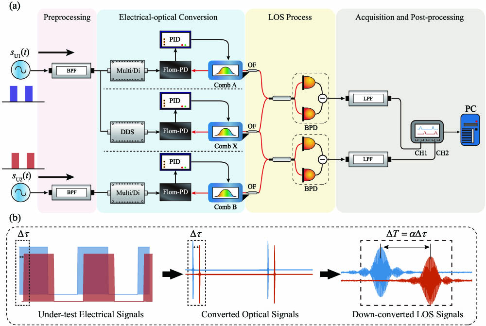
Figure 1.Schematic of the time interval measurement setup. (a) Time interval measurement setup. The two band-pass filters (BPFs) in the preprocessing part filter a certain harmonic of the under-test pulses, which serve as the combs’ reference after being multiplied, divided, or synthesized. The direct digital synthesizer (DDS) in the electrical-to-optical conversion part generates a sinusoidal wave with a slight frequency difference from its input signal. The repetition frequencies of three combs are phase-locked with the fiber-loop optical-microwave phase detector (FLOM-PD) and the PID. The outputs of combs
In the signal preprocessing phase, the system uses adjustable bandpass filters (BPFs) and frequency multipliers/dividers to obtain a single harmonic component of the input waveforms that equals integer multiples of 100 MHz for the subsequent process. Note that the phase time of every harmonic contains the same information as the original electrical signal dose [34] (see the Appendix A). Measuring the time interval of the sine signal directly by electrical means leads to the precision of the ps level [35,36]. To overcome this limitation, in the E-O conversion process, we lock the repetition frequencies of two OFCs, namely comb and comb , to the previously obtained single harmonic signals using the fiber-loop optical-microwave phase detector (FLOM-PD) technique [37–39]. In our scheme, the 2 GHz harmonic of the signal being tested is obtained and used for phase locking, and the residual phase noise after phase locking was at 1 s, as evaluated by the phase noise analyzer (Microchip Technology, 53100A). It ensures a standard deviation of less than 45 fs of the locking-induced noise of the time measurement.
In the optical domain, the system uses the state-of-the-art LOS technique to downconvert two comb signals to microwave combs with times precision improvement (see the Appendix A). The key parameter quantifies the stretch of time scale when using a local oscillator (LO) comb [comb in Fig. 1(a)], with a slightly different frequency of , to sample the measured OFC with a frequency , yielding a microwave comb containing the time information of the measured OFC, but with higher precision. The frequency difference is achieved by a direct digital synthesizer (DDS). Here, we used two OFCs with a repetition frequency of 100 MHz as the measured OFCs (comb and ) and an OFC with a repetition frequency of 100.001 MHz as the LO-OFC, which improved the time measurement precision by times. Note that the repetition frequencies of the combs are all adjustable with a temperature controller and a PZT, enabling them to be synchronized to the signals being tested for the subsequent process.
In the LOS process, the optical part is constructed with full polarization-maintaining fiber couplers and optical filters (OFs) with a central wavelength of 1550.12 nm and a bandwidth of 0.8 nm to prevent polarization-induced amplitude fluctuation. OFs are used not only to limit the OFCs’ spectrum in the same band to obtain a stable and clear interference pattern but also to fulfill the Nyquist condition and to prevent spectrum overlapping [40]. The interference result is subsequently transformed into an electrical signal with balanced photodetectors (BPDs, Thorlabs, PDB450C) for the convenience of data acquisition and processing. Therefore, the conversion process can be summarized by first converting the electrical signals being tested to optical signals and then downconverting to the microwave LOS signals using the LOS technique, as illustrated in Fig. 1(b). In the whole process, to ensure the long-term stability of the system, we shortened the pigtails of commercial wavelength division multiplexer (WDM) devices, couplers, and other optical components and directly fused them together. We also kept the electrical cables as short as possible and implemented temperature control in the detection section to minimize the impact of internal path variations on the time measurements. The upper and lower branches of the system have a baseline delay for not precisely matching the path length, while it is calibrated before conducting the measurements.
The acquisition part contains two electrical low-pass filters (81 MHz) to obtain the frequency components introduced by the beating OFCs, and an oscilloscope (OSC, Rigol, MSO8204) is used to simultaneously acquire the data from two channels. The duration of an LOS signal in our experiment was approximately 4 μs. To fit the envelope of the LOS signal accurately, we expected at least 100 points in the pulse duration. This means that the sampling rate was expected to be over . A higher sampling rate will improve the resolution of the LOS signal (see the Appendix A), while also increasing the data processing cost. To balance the LOS signal precision and the processing speed, we set the sampling rate to 500 MHz in our experiment. A screen containing a set of the LOS waveforms is shown in Fig. 2, where two input channels of the OSC are simultaneously acquired and then delivered to the computer. These two signals contain time information of the input electrical signals, but with higher measurement precision. The timescale of the downconverted LOS signal is at the microsecond level, which can be easily acquired and processed using digital signal processing techniques, compared to the timescale of tens of picoseconds level with direct measurement. The data processing procedure is given in the Appendix A.
![]()
Figure 2.Processing of the down-converted LOS signal by the envelope calculation and localization (i.e., center finding). The process is achieved by first fitting the signal’s envelope and then calculating its center of gravity.
B. Measurement Precision
In our experiment, we assessed the precision of the time interval measurement system by generating the test signal by power-splitting a single 100 MHz square wave produced by an arbitrary waveform generator (AWG, Keysight, M8195A). As explained in Section 2.A, we applied filtering to isolate the first harmonic of the signals, which were then multiplied to 2 GHz. These resulting signals served as the references for comb and comb , respectively. Hence, the time interval of two square waves under test was transformed into the measurement of two downconverted LOS signals. In our scheme, we measured the interval by calculating the LOS envelopes’ center of gravity, as shown in Fig. 2, and the calculated result is shown in Fig. 3(a). With continuous acquisition, the time interval could be displayed and plotted in real time. The black circles stand for the raw measured data, with the average value being and the standard deviation being 83 fs. To further improve the precision, we also optimized the system’s performance with a Kalman filter in real time. The red dots stand for the processed data with the Kalman filter, with the standard deviation being 28 fs.
![]()
Figure 3.Measurement results of system’s precision. (a) Measurement results of the time difference. Black circles represent raw data, while red points represent data processed with the Kalman filter. (b) Measurement precision of the data. Blue crosses indicate the precision of a commercial time-interval counter (Keysight, 53230A). Black circles represent the precision of our work with raw data, while red points represent the precision of our work with processed data.
To further reduce the system noise, we also considered averaging the sampling results to obtain the optimized results. Here, we used the standard error of the mean (SEM) to estimate the precision after averaging, given by
Furthermore, our scheme can measure the time interval of periodic signals with arbitrary waveforms. To demonstrate this, we generated sine waves, square waves, and triangular waves using the AWG. The consistent measurement results presented in Fig. 4 provide evidence to support this claim.
![]()
Figure 4.Measurement precision (processed data) of the system using 100 MHz sine waves, square waves, and triangular waves. The result shows similar measurement precision for the different waveforms.
The precision was achieved via 100-times acquisition, data transmission, and data processing, and it took approximately 1 s per cycle, with time being mainly consumed in the transmission part. When the OSC was replaced with a high-speed acquisition card, the system achieved 1000 LOS scans of output per second, and the fs-level precision was realized in 0.1 s.
C. Key Parameters Analysis
To investigate the noises introduced by different components, we analyzed the key elements influencing our system’s performance. The system’s performance was limited by various factors, including the synchronization precision of combs and from the signal being tested, the amplitude noise from the detectors, and the sampling rate.
The amplitude noise and sampling rate affected the system precision during the localization process. To investigate their influence in detail, we simulated them with the LOS model described in the Appendix A. In our experiment, the BPD and the light source introduced amplitude noise with a standard deviation of 7 mV, which is approximately 1.32% of an LOS pulse, and we denote it as the relative intensity noise (RIN). The RIN affects the localization process and thus brings a fitting error to the measurement result, as shown in Fig. 5(a). We used 1.32% Gaussian white noise added on an LOS signal’s amplitude to simulate the system’s performance. The sampling rate was set to 500 MHz, as determined by the experimental parameters, and the standard deviation of the calculated time interval fluctuation was 19 fs [see Fig. 5(b)].
![]()
Figure 5.Simulation results of the effect of the relative intensity noise (RIN)-induced time fluctuation. (a) The RIN affects the localization process and brings fitting errors. (b) The time fluctuation is caused by 1.32% RIN, where the sampling rate is set to 500 MHz corresponding to the experimental parameter. (c) The relation of RIN-induced time fluctuation,
Note that the influence of the RIN was tightly connected, with both the (carrier-envelope offset frequency; see the Appendix A) difference between the two combs of an LOS signal and the sampling rate of the OSC. Because the of the combs are all free-running, it is crucial to choose an appropriate sampling rate to reduce the influences brought by the drift of the and also consider the processing speed. For that purpose, we simulated the relation of the RIN-induced time fluctuation, the -difference, and the sampling rate for a fixed RIN level 1.32%, and the results are shown in Fig. 5(c). The axis ranges from 0 to 50 MHz because of the 100 MHz repetition frequency of the combs; a larger is practically equivalent to because of the periodicity of the combs’ spectrum.
The results of Fig. 5(c) illustrate that when the sampling rate was larger than the repetition frequency (namely, 100 MHz), the RIN-induced time fluctuation was not evidently related to . The higher the sampling rate is, the lower the noise that would remain. The 500 MHz sampling rate in our experiment led to 16–20 fs noise, as shown in Fig. 5(d), which is relatively low compared to the phase-locking-induced noise. If the sampling rate was below 100 MHz, the time interval fluctuation level would be affected because of the varying of the combs. When the was around a half-integer multiple of the sampling rate, the noise significantly increased because of the inaccurate sampling of the pulse. In addition, when the sampling rate fell lower, the noise level of other points also gradually increased because the amplitude fluctuation cannot be effectively averaged out with so few points. Moreover, to further improve the localization precision, increasing the optical bandwidth of the OF and equivalently decreasing the pulse width could potentially make a significant contribution.
According to the system’s model given in the Appendix A, the measurement noise floor was mainly composed of the residual phase noise introduced by phase locking, and the RIN-induced time fluctuation, which is
Interestingly, in Fig. 5(c), for some fixed , there were still low sampling rate regions with relatively low RIN-induced time fluctuations. For instance, if the could be manually controlled to 0 Hz, the regions that have large noise (the green regions) could be avoided, even with low sampling rates, as shown in Fig. 5(e). In this situation, the sampling rate of 100 MHz was sufficient to achieve RIN-induced noise below 40 fs (below the phase-locking-induced noise), although the system complexity would worsen. It is noteworthy that the oscillations observed in Figs. 5(d) and 5(e) are likely a result of the manually added Gaussian noise. Therefore, our focus lies in the overall magnitude rather than the specific values of individual data points.
For future studies, since the RIN-induced localization noise is at a relatively low level and has limited influence on the system performance at this stage, we did not conduct further in-depth research on this aspect and experimentally treated it as a known factor; the experimentally measured value is 1.32%. However, it is a complex composite consisting of at least analog–digital conversion quantization accuracy, detector electrical noise, and shot noise. It will be an important theoretical question to be analyzed and calculated after improving the accuracy of the light source locking.
In other aspects, the update rate (equal to ) is also a crucial consideration in some applications. It can be increased by simply enlarging . However, it cannot be infinitely large, considering the LOS amplification factor and the Nyquist bandwidth. Exploring the trade-off between these factors would be a valuable area for further research.
D. Discussion
In this study, with the optical mean (namely, the LOS technique), we achieved a high-precision and simple time interval measurement setup that can drastically promote the precise measurement of electrical signals. For demonstration, we built a CEO-free system to meaure the time interval of two squared electrical signals, and simulations were implemented to optimize the experimental parameters. Experimentally, we achieved 83 fs in a single-LOS-scan precision, and we further approached 3.05 fs with data processing, which is about three orders of magnitude better than the result of traditional time interval counter methods.
Compared to traditional direct detection of the time interval, our method has the advantage of avoiding the ambiguity brought by the rising edge of a pulse, creating the potential for the time interval measurement of arbitrary waveform pulsed signals. The possible restrictions of the performance were also discussed theoretically, and they can guide us toward further optimization of the setup. In our approach, the measurement is performed by synchronizing the combs with the periodic signals under test. As a result, we are currently unable to measure the time interval between individual pulses, and this aspect is left for future investigation. Based on our work, a real-time high-precision time interval measurement system can be developed to achieve sub-fs measurement, which we believe will open a new pathway for high-precision metrology, such as ultrahigh precision navigation and time synchronization.
APPENDIX A: METHODS
The LOS technique is achieved by the interference between three OFCs, whose spectrum comprises a series of narrow bandwidth lines with the frequency , which can be written as , where represents large integers (typically with the order of , with being in an optical region). Moreover, denotes the repetition frequency, and is the carrier envelope offset (CEO) frequency, which is related to the carrier and envelope phase offset. In the time domain, a pulse train with a short duration and a period of is generated by an OFC, and the ultralow noise timing jitter is usually obtained by locking its phase to a reference oscillator. High time resolution measurement benefits from sampling one OFC signal with another OFC that has a slight repetition frequency offset . The effective time measurement result is theoretically optimized by a magnifying factor . Specifically, the envelope phase variation of each comb is enlarged and revealed on the macroscopic signal with the relation
Self-developed SESAM-based OFCs are built with a 1560 nm central wavelength and 12 nm line width. The repetition frequency is approximately 100 MHz, which is adjusted by a piezoelectric ceramic transducer (PZT) with a bandwidth of 100 Hz, an optical delay line with an adjustable range up to 1 MHz and a 100 Hz step, and a temperature-controlling plate with a 10 K temperature-controlling range and 0.001 K precision.
The OFCs have 100 mW of output power, which is achieved with a built-in erbium-doped fiber amplifier (EDFA). The high output power ensures that the energy is sufficient for the subsequent operations, including phase locking, interference, and monitoring. The polarization of the OFCs is stabilized with polarization controllers for the stability of the interference. The CEO frequency of the combs does not need to be controlled, so the system complexity can be significantly reduced.
To achieve the fs precision time interval measurement, we expect the phase of the electrical signals being tested to be transferred to the corresponding OFCs precisely to employ the follow-up LOS technique; then, we can expect the interval of the combs to be stretched by LOS and precisely measured based on the combs’ high time resolution characteristics. The signal preprocessing procedure aims to filter (together with multiplying/dividing) a single frequency component with no phase distortion, which can serve as the reference oscillator of combs and .
Assume that two arbitrary signals have the forms given by
Note that for arbitrary waveform signals, different harmonics have different energies. For situations where direct filtering of the high-order harmonic is not feasible, an alternative approach is to obtain it by multiplying the first-harmonic signal, which typically possesses the highest energy. Furthermore, because the introduced time interval resulting from optical-microwave synchronization using FLOM-PD is unaffected by the power levels of the electrical signal, harmonic energy differences will not influence subsequent experiments. This characteristic enables our scheme to measure different waveform signals or use different frequency components without compromising the measurement results.
To fully use the high time resolution characteristic of OFCs, we must ensure that the OFCs carry the time information of the electrical signals under test by phase-locking techniques. To realize high-precision phase locking, we use the FLOM-PDs, whose noise property surpasses the traditional mixer technique [
For data processing, the LOS signals’ envelopes ( is the signal number) carry the time information of the signals under test, so they are preliminarily extracted with the Hilbert transformation
Conventionally, the delay can be extracted with curve-fitting on the envelope and peak-finding, while the line shape of the LOS envelope depends on the OFCs’ mode-locking process and needs optimization for different OFCs, such as hyperbolic secant fitting for an LOS signal generated by two soliton mode-locked lasers. If the gain narrowing effect of the amplifiers is considered, the line shape can be approximated to Gaussian [
Additionally, a full scan of the LOS waveform covers multi-ns oscillator time and most of it measures baseline. To improve the efficiency of our scheme, we implemented a threshold-based approach. If a data point is determined to be a baseline, instead of recording it, we increase the index of the data, thus optimizing the data processing speed in our implementation. Optimizing the measurement duty cycle would be another effective way, by using, e.g., time-programmable frequency combs [
To give a further explanation of our system, one can consider the signal of comb and comb in a specific optical channel (about 0.8 nm in width). Both combs are composed of comb teeth, and the fluctuations of their repetition frequency and CEO frequency are considered. The signal of comb can be written as
This means that the measured single LOS signal frequency stability is determined by the relative repetition frequency fluctuation of comb , comb , and the enlargement factor .
Together with the LOS signal of comb and comb , the relative fluctuation of their phase time difference (that is, the system limit) can be written as
In addition, from Eqs. (
Over and above that, Eq. (
References
[9] Q. An. Review of methods and techniques of precise time interval measurements for particle physics experiments. Nucl. Tech., 29, 453-462(2006).
[20] S. Henzler. Time-to-Digital Converter Basics(2010).
[21] X. Ren, X. F. Zhang. Methods of high precision time-interval measurement. 4th International Conference on Electronic Information Technology and Computer Engineering (EITCE)(2020).
[23] D. W. Allan, H. Daams. Picosecond time difference measurement system. Symposium on Frequency Control(1975).
[31] M. Kajima, K. Minoshima. A simple optical-zooming positioning system using a femtosecond frequency comb. Conference on Lasers & Electro-Optics(2009).
[34] G. Marra. Transfer of optical frequency combs over optical fibre links(2013).
[36] Z. Jin, Y. Xu, D. Yu, B. Luo, Z. Chen, G. Wu, H. Guo. Analyzing the influence of InGaAs photodetectors in comb-based frequency transfer. Frontiers in Optics + Laser Science(2022).
[41] G. P. Agrawal. Nonlinear Fiber Optics(2000).

Set citation alerts for the article
Please enter your email address
© Copyright 2018-2021 | Chinese Laser Press. All Rights Reserved 沪ICP备15018463号-20