
Meirui Chen, Lü Jiang, Hongmin Mao, Huijuan Sun, Jiantao Peng, Guoding Xu, Lifa Hu, Huanjun Lu, Zhaoliang Cao. High-Precision Static Aberration Correction Method of SPGD Algorithm[J]. Acta Optica Sinica, 2023, 43(5): 0511001
- Acta Optica Sinica
- Vol. 43, Issue 5, 0511001 (2023)
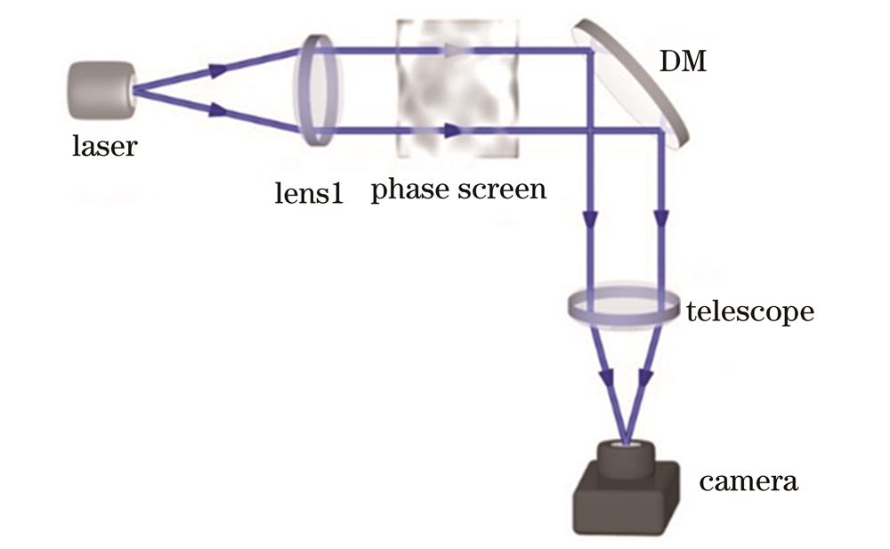
Fig. 1. Optical path for static aberration correction
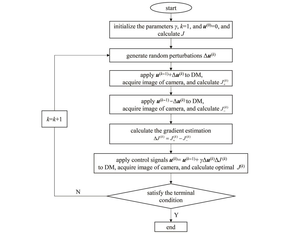
Fig. 2. Flow chart of SPGD algorithm
Fig. 3. Scheme of performance metrics combination method
Fig. 4. Flow chart of performance metrics combination method
Fig. 5. Simulated results of distorted image. (a) First 36 Zernike coefficients; (b) distorted wavefront; (c) far-field intensity distribution
Fig. 6. Far-field intensity distributions after EE correction. (a) DEE=0.5d; (b) DEE=d; (c) DEE=1.5d; (d) DEE=2d; (e) DEE=2.5d; (f) DEE=3d
Fig. 7. Intensity distributions of horizontal centerline of target surface. (a) DEE=0.5d; (b) DEE=d; (c) DEE=1.5d; (d) DEE=2d; (e) DEE=2.5d; (f) DEE=3d
Fig. 8. Relationship between corrected SR and encircled diameter
Fig. 9. Correction results for MR. (a) Convergence curve; (b) residual wavefront; (c) far-field intensity distribution
Fig. 10. Corrected results of MR method for 10 times repetition. (a) SR; (b) RMS of residual wavefront
Fig. 11. Performance metric convergence curve of combination method
Fig. 12. Comparison of simulation correction results. (a)-(c) Residual wavefront; (d)-(f) far-field intensity distributions; (g)-(i) intensity distributions of horizontal centerline of target surface
Fig. 13. Comparison of different noise simulation correction results. (a)-(d) Weak noise with gray level of 80; (e)-(h) strong noise with gray level of 1200
Fig. 14. Correction results of EE, MR, and performance index combination method for different noises
Fig. 15. Correction results of EE method and performance index combination method for different encircled diameters. (a) SR; (b) RMS of residual wavefront
Fig. 16. Correction results of multiple random static aberrations. (a) SR; (b) RMS of residual wavefront
Fig. 17. Optical path of static aberration correction system
Fig. 18. Experimental results of static aberration correction. (a)-(d) Images of point object; (e)-(h) intensity distributions in center line of images
Fig. 19. Performance metric convergence curves. (a) EE method; (b) MR method; (c) performance metric combination method
|
Table 1. Parameters in simulation

Set citation alerts for the article
Please enter your email address
© Copyright 2018-2021 | Chinese Laser Press. All Rights Reserved 沪ICP备15018463号-20