
Rumao Tao, Long Huang, Pu Zhou, Lei Si, Zejin Liu. Propagation of high-power fiber laser with high-order-mode content[J]. Photonics Research, 2015, 3(4): 192
- Photonics Research
- Vol. 3, Issue 4, 192 (2015)
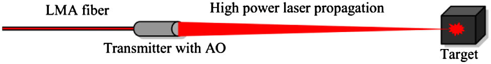
Fig. 1. Scheme of the launch of LMA fiber laser.
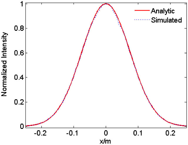
Fig. 2. Comparison between the analytic and simulated results when z = 1 km C n 2 = 1 × 10 − 15 m − 2 / 3
Fig. 3. Irradiance distribution of fiber modes. (a) LP 01 LP 11
Fig. 4. Irradiance distribution at z = 5 km A L P 11 = 0 A L P 11 = 0.3 Δ ϕ = π / 4 A L P 11 = 0 A L P 11 = 0.3 Δ ϕ = π / 4
Fig. 5. Normalized intensity distribution.(a) A L P 11 = 0.1 z = 5 km A L P 11 = 0.1 Δ ϕ = π / 4 A L P 11 = 0.2 z = 5 km A L P 11 = 0.2 Δ ϕ = π / 4 A L P 11 = 0.3 z = 5 km A L P 11 = 0.3 Δ ϕ = π / 4 Δ ϕ = π / 4 z = 5 km
Fig. 6. PIB as a function of relative phase and HOM content A L P 11 z = 5 km Δ ϕ = 0
Fig. 7. PIB as a function of Δ ϕ
Fig. 8. Example of phase screen used in numerical simulation. (a) C n 2 = 5 × 10 − 16 m − 2 / 3 C n 2 = 1 × 10 − 15 m − 2 / 3
Fig. 9. Irradiance distribution at z = 5 km A L P 11 = 0.3 Δ ϕ = π / 4
Fig. 10. Normalized intensity distribution. (a) A L P 11 = 0.2 Δ ϕ = π / 2 A L P 11 = 0.2.
Fig. 11. PIB as a function of HOM content A L P 11
Fig. 12. PIB as a function of turbulence strength.
Fig. 13. SI as a function of turbulence strength.
Fig. 14. PIB as a function of Δ ϕ C n 2 = 1 × 10 − 16 m − 2 / 3 C n 2 = 5 × 10 − 16 m − 2 / 3 C n 2 = 1 × 10 − 15 m − 2 / 3

Set citation alerts for the article
Please enter your email address
© Copyright 2018-2021 | Chinese Laser Press. All Rights Reserved 沪ICP备15018463号-20