Automated segmentation of optical coherence tomography images

C. Kharmyssov; M. W. L. Ko; J. R. Kim

doi:10.3788/COL201917.011701

Abstract

We propose a fast and accurate automated algorithm to segment retinal pigment epithelium and internal limiting membrane layers from spectral domain optical coherence tomography (SDOCT) B-scan images. A hybrid algorithm, which combines intensity thresholding and graph-based algorithms, was used to process and analyze SDOCT radial scans (120 B scans) images obtained from twenty patients. The relative difference in position of the layers segmented by the proposed hybrid algorithm and by the clinical expert was 1.49% ± 0.01%. The processing time of the hybrid algorithm was 9.3 s for six B scans. Dice’s coefficient of the hybrid algorithm was 96.7% ± 1.6%. The proposed hybrid algorithm for the segmentation of SDOCT images had good agreement with manual segmentation and reduced processing time.

Image analysis and segmentation of optic nerve head (ONH) structures is important for understanding the mechanism of retinal ganglion cell degeneration in glaucoma and the development of new diagnostic approaches and treatments^[1]. Spectral domain optical coherence tomography (SDOCT) is a noninvasive imaging modality, which generates optical cross-sectional images of the retina and ONH. Segmentation of the ONH structures, however, is challenging.

Application of image analysis algorithms into clinical use is a major challenge due to their overall complexity^[2]. An application of the SDOCT medical image analysis into clinical use requires several actions: (1) validate the automated algorithm if the gold standard has not been renowned, (2) select suitable values for image parameters and algorithms to design the specific optical coherence tomography (OCT) clinical data, and (3) run the algorithm with suitable parameters to set specific properties of the input data^[2].

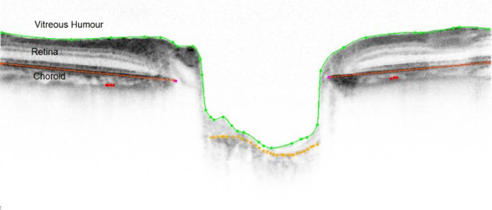
The internal limiting membrane (ILM) (solid green line in Fig. 1) forms a membrane between the retina and the vitreous. Retinal thickness is a measure of the distance between the ILM and retinal pigment epithelium (RPE)^[3]. A number of segmentation methods have been suggested for the automatic segmentation of OCT images related to its dimension. One-dimensional (1D)-based approaches find gradient peaks (intensity thresholding algorithm) through the layer boundary^[4–7]. Two-dimensional (2D)-based methods determine the retinal layers using 2D image segmentation methods, such as level sets and edge detection^[8–11]. Three-dimensional (3D)-based methods segment the retina layers based on a graph-based approach^[12–14]. The latter is proved to be a robust technique to segment layers, however, it is computationally demanding.

Sign up for Chinese Optics Letters TOC. Get the latest issue of Chinese Optics Letters delivered right to you！Sign up now

Figure 1.SDOCT image with retinal pigment epithelium layers (RPE, solid red line), internal limiting membrane (ILM, solid green line), and choroid representation.

Segmentation is a crucial part of OCT image analysis. Characteristic features of ONH changes in glaucoma include loss of retinal ganglion cell axons in the region of prelaminar neural tissue (retina). The retina can be reconstructed in 3D and embedded to sclera for characterization of ONH biomechanical environment^[15]. Girard et al.^[16] manually segmented and automatically reconstructed nine glaucoma patients to establish associations between retinal sensitivity and ONH strain. Therefore, development of an automatic ONH retinal layer segmentation algorithm for SDOCT images is beneficial, as manual labeling of the layers is time-consuming and a subjective operation.

The intensity thresholding algorithm requires only a short processing time. However, it may not be able to locate the entire retinal layer, particularly in the distorted image region due to the indistinguishable local maxima/minima (i.e., break). The graph-based algorithm can segment the critical regions continuously, however, it requires a long processing time. This study aims to develop a hybrid segmentation algorithm. This will be achieved by increasing the segmentation accuracy and reducing the segmentation processing time by combining intensity thresholding and graph-based algorithms. In this Letter, the accuracy of the proposed hybrid algorithm and its reproducibility on retina thickness measurement are investigated, and the results are compared with intensity thresholding and graph-based algorithms.

The major contribution of this work is twofold. (1)To present an extended and novel version of the graph-based algorithm introduced by Chiu et al.^[14], which segments the macula region. This method can be applied to segment ONH regions based on intensity thresholding and the graph-based approach to fill the indistinguishable local maxima/minima.(2)A faster segmentation algorithm is presented that is able to segment two key layers (ILM and RPE) from the ONH region. Automatic segmentation in a short time in such high-resolution datasets reflects an important contribution.

The ONH region was imaged with the Spectralis OCT (super-luminescent diode laser center wavelength, 870 nm; scan speed, 40,000 A scans per second; Heidelberg Engineering, Heidelberg, Germany) in six sections of radial 1024 A scans at 30° angles. Cross-sections of A scans were positioned at the center of the ONH manually by the operator, using the eye tracking system to estimate the clinical disc margin. The image signal-to-noise ratio was increased with automatically averaging software of fifteen B scans. The scan quality score of each image was at least equal to 20. The OCT data sets were collected from 20 patients recruited for a study investigating lamina cribrosa and ONH deformation in glaucoma^[1,17].

A total of 20 patient SDOCT scans (120 B scans) were included in this study. The resolution of the images is $1024 \times 400$ . The OCT images were manually segmented by a clinician using a custom software developed in MATLAB (R2016 b, MathWorks, Inc.) to serve as a reference standard for evaluation of the agreement of the proposed hybrid segmentation algorithm (Fig. 1).

First, the ILM and RPE layers were segmented by the intensity thresholding algorithm. However, the intensity values varied within columns, and therefore, continuous detection of points with the thresholding technique was challenging, especially in diseased eyes. The graph-based algorithm^[14,18] was then used to further process the image to ensure a continuous segmentation of labeling lines.

The processing of a single image by using only the graph-based algorithm took a substantial amount of time to segment the entire layer (421 s, computed with a computer with CPU i5 core 6.60 GHz, 4 GB RAM) due to the high resolution of the image and high computational power demand of the algorithm. The processing time of 100 images would take up to several hours; hence, it is not applicable to daily routine clinical imaging and diagnosis. Therefore, the proposed hybrid algorithm aims to combine the intensity thresholding method with the graph-based algorithm to decrease computational processing time while maintaining good segmentation accuracy.

Sections A to E describe the proposed hybrid segmentation algorithm. The schematic overview of the proposed hybrid algorithm is shown in Fig. 2.

Figure 2.Overview of automatic segmentation of the ILM and RPE layers in SDOCT images.

A. Preprocessing: To suppress the thermal and electronic noise, the original SDOCT image indicated as $I (x, y)$ for $(x, y) \in [1, N_{c}] \times [1, N_{r}]$ , where $N_{c}$ is the number of columns, and $N_{r}$ is the number of rows, was first convolved with a 2D Gaussian smoothing kernel with a standard deviation of two, which is a common filtering method that the authors of Refs. [1,19,20] used for B-scan modes. The image was then convolved with a $10 \times 10$ median filter by linear low pass filtering averaging across edges. The image after the combination of these two filtering methods, denoted as $\hat{I} (x, y)$ , gave adequate segmentation results with suppressed local image speckle.

B. Intensity-based algorithm: The principle of finding the RPE layer was based on the intensity of the backscattered light appearing as the lowest compared with other layers. It is easily visible and easy to detect, so the pixels with the lowest intensities in the A scans were assigned as the boundary of RPE, denoted as $L_{RPE}$ and defined by the local minima point, $L_{RPE} = {(x, y_{RPE}) | x \in [1, N_{c}], y_{RPE} = \min [\hat{I} (x, u)]},$ (1)where $u \in [1, N_{r}]$ , and it is related to the intensities of the de-noised image $\hat{I}$ in the corresponding column. To distinguish the points caused by noise and blood vessels, a fourth-order polynomial, $f_{BM} (x) = {\tilde{p}}_{4} x^{4} + {\tilde{p}}_{3} x^{3} + {\tilde{p}}_{2} x^{2} + {\tilde{p}}_{1} x + {\tilde{p}}_{0}$ , was used to create a smooth and continuous curve to eliminate randomly appearing RPE points (leave it empty) as a result of abrupt transitions of the delineated boundary. The principle of finding ILM is based on automatically performing clustering-based image thresholding^[21].

C. Search region limitation: The outlier structures with analogous characteristics often prevent the algorithm from accidentally segmenting the outer plexiform layer (OPL) and inner plexiform layer (IPL) instead of RPE. It is beneficial to limit the search region to a valid target region, which helps to exclude any external layers. The intensity-based algorithm, described in section B, has limitations when finding the RPE boundary, where empty spaces need to be fulfilled (Fig. 3). These empty spaces were used to limit the search region in the form of a box with five pixels up and five pixels down from the start (where the gap begins) and end (where the gap ends) points of the RPE empty areas. Considering the mentioned drawbacks, the pixels, which could not be delineated by the intensity-based algorithm or wrongly delineated, were demarcated afterward by the graph-based algorithm.

Figure 3.Example of the ILM layer (blue line) and RPE layer (red line) segmentation with the solely intensity-based algorithm.

Start and end points were selected and estimated from the specific layer. This endpoint selection was performed at two ends of the image. So, if the empty part of the segmentation line is in the beginning or in the end, then an extra column of nodes is added to both sides of the image. Minimal weights were assigned arbitrarily to the intensity values in the vertical direction. Once it was segmented, the additional columns were removed. As the RPE layer represents the darkest line, it had a lower weight as a function of pixel intensity.

D. Graph weights calculation: The minimum weighted path was found using Dijkstra’s algorithm^[22] to find the associated with edges connecting two endpoints of graphs. A set of pixels in each image was characterized as an undirected graph of nodes $G = (V, E)$ , where every pair of the nodes formed an edge in the image space. The key to accurately cut graphs is to set up weights on the edges, connecting nodes according to their similarity. Borders of the objects to be segmented are given lower weights to separate it from other features of that object.

Graph weights in the literature^[23] represented intensity variation and geometric distance. Weights were assigned to individual edges to reflect the possibility that two pixels belonged to the same line. The SDOCT images used in this study had a relatively high resolution. As a result of plane change between adjacent pixels, each node is related to its eight neighboring pixels and is disassociating with geometric distance weights. The type of graph was defined to be undirected to half of the adjacency matrix size: $w_{a b} = 2 - (g_{a} + g_{b}) + w_{\min},$ (2)where $g_{a}$ is the vertical image gradient of point $a$ , $g_{b}$ is the vertical image gradient of point $b$ , $w_{\min}$ is the minimum weight in the graph, which is equal to $10^{- 5}$ extra numbers for system stabilization, and $w_{a b}$ is the weight of lines connecting vertices $a$ and $b$ . After construction of the adjacent matrix and graph $G$ with appropriately weighted nodes with minimum total length, the empty parts, as shown in Fig. 3, were cut by using Dijkstra’s algorithm^[22]. Equation (2) shows weight calculations based on intensity gradients. It assigns high values to node pairs with low vertical gradients, where $g_{a}$ and $g_{b}$ are stabilized in the range of values between 0 and 1. Segmented images with the hybrid algorithm are shown in Fig. 4, which combines intensity-based and graph-based algorithms.

Figure 4.Segmentation result of RPE (red line) and ILM (blue line) of the hybrid algorithm, which is solely a combination of intensity and graph-based algorithms after filling RPE gaps with the graph-based approach.

E. Dice’s coefficient and segmentation errors: Three performance metrics, including Dice’s coefficient, automatic and manual relative segmentation difference (AMRSD), and relative segmentation proportion percentage (RSPP), were used to evaluate the accuracy of the algorithms compared to the manually segmented layer profile.

The distance between the upper (ILM) and lower (RPE) boundaries is represented as total retinal distance (TRT) and used as a reference standard to evaluate the accuracy of the automatic algorithm^[24]. The manually labeled TRT region between ${ILM}^{0}$ and ${RPE}^{0}$ represents the reference standard, denoted as ${TRT}^{0}$ .

Dice’s coefficient ( ${Dice}_{TRT}$ ) is used as a performance metric to evaluate the variability of the whole profile of the algorithms with the manually ground truth expert segmented image results, and it was defined as ${Dice}_{TRT} = \frac{2 | TRT \cap {TRT}^{0} |}{| TRT | + | {TRT}^{0} |} .$ (3)

The high value of ${Dice}_{TRT}$ indicates a lower difference with the results from manual segmentation, thus better performance of the automatic algorithm^[25].

AMRSD was defined as the relative segmentation error of whole profile between ${RPE}^{0}$ (manually segmented layer) and RPE (automatically segmented layer). A higher value of AMRSD represents a higher relative error: ${AMRSD}_{RPE} = | {RPE}^{0} - RPE | \times 100 % .$ (4)

RSPP calculates the number of the ${ILM}^{0}$ and ${RPE}^{0}$ points relative to automatically segmented RPE and ILM that can be segmented by the hybrid algorithm, intensity thresholding algorithm, and graph-based algorithm, defined as the ratio of the total number of RPE (TNRPE) and total number of automatically segmented ILM (TNILM) pixels to manually segmented values ( ${TNILM}^{0}$ and ${TNRPE}^{0}$ ). The higher value of RSPP represents more data points (pixel) to be segmented by an automatic algorithm: ${RSPP}_{RPE} = \frac{TNRPE}{{TNRPE}^{0}} \times 100 %,$ (5) ${RSPP}_{ILM} = \frac{TNILM}{{TNILM}^{0}} \times 100 % .$ (6)

One hundred twenty SDOCT B scans of twenty glaucoma patients were included for analysis. For each SDOCT B scan, the RPE and ILM layer boundary pixels were first labeled manually by a clinician.

The performance of automated segmentation obtained with the three algorithms (intensity thresholding algorithm, graph-based algorithm, and proposed hybrid algorithm) was compared with the 120 manually segmented layer profiles. Figure 1 shows the manually segmented layer profile outlined by a clinician, and Fig. 4 shows the automated segmentation results of the hybrid algorithm from a selected patient.

The average processing time, AMRSD, and Dice’s coefficient are summarized in Table 1. As shown in Table 1, the intensity thresholding algorithm was 9.27 times faster than the graph-based algorithm and the hybrid algorithm. AMRSD for the intensity thresholding algorithm and the proposed hybrid algorithm fell in a similar range and had a comparable value, whereas the graph-based algorithm showed the highest AMRSD.

Algorithm	Processing time (s)	AMRSD (µm)	Dice’s coefficient (%)
Intensity thresholding algorithm	3.7	5.42±0.03	96.8±1.7
Graph-based algorithm	34.3	24.7±0.23	74.1±14.8
Proposed hybrid algorithm	9.3	5.73±0.03	96.6±1.6

Table 1. Summary of the Processing Time of One Image, Mean and Standard Deviation of ILM and RPE Comparison of Relative Difference with Manually Segmented Image, and Dice’s Coefficients of 120 Images

View all Tables

Dice’s coefficient of the graph-based algorithm was considerably lower, compared with Dice’s coefficient of the other two algorithms ( $> 96 %$ ) and had a value of $74.1 % \pm 14.8 %$ . There were no detectable differences in Dice’s coefficients between hybrid and intensity thresholding algorithms.

Table 2 shows the summary of RSPP, which varies across RPE and ILM layers. RSPP results for RPE and ILM with the intensity thresholding algorithm were $52.2 % \pm 18.5 %$ and $84.6 % \pm 12.8 %$ , respectively. The intensity algorithm could segment about only half of the RPE points with more segmented pixels for ILM. Slightly larger RSPP was noted for the graph-based algorithm compared with the intensity thresholding algorithm, which segmented about the same amount of points for RPE and ILM. The largest RSPPs of the RPE and ILM were noted in the proposed hybrid algorithm.

Algorithm	RPE^a	ILM^a
Intensity thresholding algorithm	52.2±18.5	84.6±12.8
Graph-based algorithm	76.9±15.9	76.9±12.4
Proposed hybrid algorithm	88.3±9.5	88.5±9.8

Table 2. Summary of RSPP Comparison for RPE and ILM Layers of 120 Images

View all Tables

ONH surface depth (ONHSD) (green lines) represents the average perpendicular distances from a line joining Bruch’s membrane opening (BMO) points (red points and brown line) to the ILM surface (blue line) (Fig. 5). ONHSD was calculated as an average for the analysis. ONHSD agreement between the manually detected surface (i.e., ILM layer) and the proposed hybrid algorithm is shown in the Bland–Altman^[26] plot in Fig. 6. The average difference of ONHSD was $1.58 % \pm 1.87 %$ , which shows good agreement between the manually traced and automatically delineated surfaces.

Figure 5.Depiction of the ONHSD, which represents an average of perpendicular distances from a red line joining two BMO points to the ILM layer.

Figure 6.Bland–Altman plot of the ONHSD measurement between the proposed hybrid algorithm and manual segmentation.

The graph-based approach^[27–29] for the segmentation of SDOCT images is an efficient algorithm that warrants total optimality of the results with respect to the cost function. High resolution and a large number of SDOCT images require substantial computational power and processing time for the calculation. The processing time with the graph-based algorithm could be reduced in multiple ways. In this study, a hybrid algorithm was proposed, which integrated the ability to incorporate a fast and simple intensity thresholding algorithm and the robustness of the graph-based approach in the presence of noise, as well as disease induced disruptions. The aim of this study is to increase segmentation accuracy and reduce the computational processing time for the segmentation of RPE and ILM layers in the SDOCT images.

The results show the hybrid algorithm is accurate and reproducible. The processing time of the graph-based algorithm (34.3 s) was about four times slower than the average processing time of the proposed hybrid algorithm (9.3 s), and the intensity thresholding algorithm required 3.7 s, which was the fastest algorithm among these three algorithms. However, 52% of data points of the RSPP of the intensity thresholding could be segmented by the intensity thresholding algorithm compared with the manually segmented ILM layer profile. The RSPP of the proposed hybrid algorithm showed the highest value in both ILM and RPE layers compared to the intensity thresholding algorithm and graph-based algorithm ( $both > 88 %$ ).

AMRSD of the proposed hybrid algorithm ( $5.73 \pm 0.03 µm$ ) was lower than that of the graph-based algorithm ( $24.7 \pm 0.23 µm$ ) and showed a comparable value with that of the intensity algorithm. The proposed hybrid algorithm assumes the RPE layer is continuous. However, this layer can be distorted by disease and artifacts. The algorithm can digress from the RPE layer, which results from gradient changes instead of smooth segmentation.

Dice’s coefficient of the proposed hybrid algorithm is $96.6 % \pm 1.6 %$ , which shows substantially higher consistency with the manually segmented image in comparison with the graph-based algorithm ( $74.1 % \pm 14.8 %$ ). The proposed hybrid algorithm robustly segmented both the RPE and ILM layers in SDOCT images. This method has certain limitations when applied to the RPE segmentation task for finding BMO points. Dice’s coefficients varied through different images due to different image noise levels. Dice’s coefficient standard deviation was 1.6 among the images. The variability of the graph algorithm was significantly lower, showing a standard deviation of 14.8.

SDOCT imaging has shown to be effective for the quantitative study of retinal structures in human retinas. Intra-retinal layer segmentation is important for aiding in a better understanding of the pathophysiology of systemic diseases^[27]. The proposed hybrid algorithm shows a high degree of accuracy and faster processing time, thus, making it more preferable for noninvasive quantification of human retinal layers in clinical analysis. The hybrid algorithm [Fig. 7(b)] could recognize and segment nearly invisible and exceedingly low contrast ILM layers from a primary open-angle glaucoma patient [red box, Fig. 7(a)] SDOCT image. In addition, the hybrid algorithm could recognize the RPE layer from two-level high contrast layers [green box, Fig. 7(a)].

Figure 7.Illustration of the (a) raw image of ONH from SDOCT of a primary open-angle glaucoma patient and (b) automatically segmented image with the hybrid algorithm of ILM (blue line) and RPE (red line) layers.

In summary, we have proposed and presented a fast and accurate hybrid algorithm integrating the fast and simple intensity thresholding algorithm and the robustness of the graph-based approach for the segmentation of RPE and ILM layers in SDOCT images. Comparative studies of the hybrid algorithm segmented profiles with the segmentation results from the intensity thresholding algorithm, graph-based algorithm, and manual segmentation in 120 SDOCT images showed good accuracy of 96.6%. The processing time of one image by the hybrid algorithm is 9.3 s, which is only one-fourth of the processing time required for the graph algorithm, which is a great advance in order to bring real-time image analysis into a clinical routine application.

References

[1] Z. Wu, G. Xu, R. N. Weinreb, M. Yu, C. K. Leung. Ophthalmology, 122, 1317(2015).

[2] D. C. DeBuc. Image Segmentation(2011).

[3] D. Xiang, G. Chen, F. Shi, W. Zhu, Q. Liu, S. Yuan, X. Chen. IEEE J. Biomed. Health Info., 27, 5880(2018).

[4] D. Koozekanani, K. Boyer, C. Roberts. IEEE Trans. Med. Imaging, 20, 900(2001).

[5] A. Chan, J. S. Duker, H. Ishikawa, T. H. Ko, J. S. Schuman, J. G. Fujimoto. Retina, 26, 655(2006).

[6] D. C. Fernández, H. M. Salinas, C. A. Puliafito. Opt. Express, 13, 10200(2005).

[7] M. Shahidi, Z. Wang, R. Zelkha. Am. J. Ophthalmol., 139, 1056(2005).

[8] M. Baroni, P. Fortunato, A. La Torre. Med. Eng. Phys., 29, 432(2007).

[9] D. C. Fernandez. IEEE Trans. Med. Imaging, 24, 929(2005).

[10] A. M. Bagci, M. Shahidi, R. Ansari, M. Blair, N. P. Blair, R. Zelkha. Am. J. Ophthalmol., 146, 679(2008).

[11] A. Yazdanpanah, G. Hamarneh, B. Smith, M. Sarunic. International Conference on Medical Image Computing and Computer-Assisted Intervention, 649(2009).

[12] M. Haeker, M. Abràmoff, R. Kardon, M. Sonka. International Conference on Medical Image Computing and Computer-Assisted Intervention, 800(2006).

[13] M. K. Garvin, M. D. Abràmoff, R. Kardon, S. R. Russell, X. Wu, M. Sonka. IEEE Trans. Med. Imaging, 27, 1495(2008).

[14] S. J. Chiu, X. T. Li, P. Nicholas, C. A. Toth, J. A. Izatt, S. Farsiu. Opt. Express, 18, 19413(2010).

[15] J. Qiu, X. Qian, Q. Cui, C. Mu, K. Zhang, B. Na, H. Song, H. Quan, Z. Liu. Jpn. J. Appl. Phys., 51, 067001(2012).

[16] M. J. Girard, M. R. Beotra, K. S. Chin, A. Sandhu, M. Clemo, E. Nikita, D. S. Kamal, M. Papadopoulos, J. M. Mari, T. Aung. Ophthalmology, 123, 1190(2016).

[17] M. Ko, C. Leung, T. Yuen. Global Medical Engineering Physics Exchanges/Pan American Health Care Exchanges (GMEPE/PAHCE), 1(2016).

[18] P.-Y. Teng(2013).

[19] T. C. Chen, B. Cense, M. C. Pierce, N. Nassif, B. H. Park, S. H. Yun, B. R. White, B. E. Bouma, G. J. Tearney, J. F. de Boer. Arch. Ophthalmol., 123, 1715(2005).

[20] T. Fabritius, S. Makita, M. Miura, R. Myllylä, Y. Yasuno. Opt. Express, 17, 15659(2009).

[21] N. Otsu. IEEE Trans. Syst. Man Cybernet., 9, 62(1979).

[22] E. W. Dijkstra. Numerische Mathematik, 1, 269(1959).

[23] J. Shi, J. Malik. IEEE Trans. Pattern Anal. Mach. Intell., 22, 888(2000).