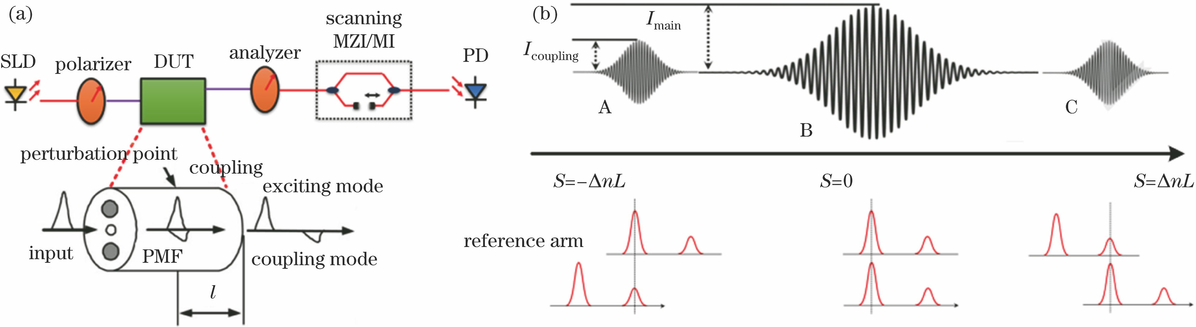
Fig. 1. Schematic of OCDP technology. (a) OCDP system; (b) typical result of OCDP system

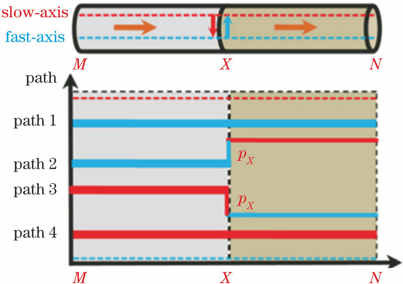
Fig. 2. Schematic of optical path tracking method

Fig. 3. (a) White light interferometer with power attenuator; (b) relationship between SNR degradation and light power of reference arm

Fig. 4. (a) Balanced detection optical path; (b) relationship between theoretical SNR and splitting ratio of coupler 1[34]

Fig. 5. (a) Schematic of PBS-calibrated method; (b) comparison between results of PBS-calibrated method and traditional method

Fig. 6. (a) Structure of differential optical delay line; (b) comparison of insertion loss fluctuation between differential structure and single GRIN lens

Fig. 7. (a) Schematic of range extention of optical delay line; (b) self-calibration signals after range extention of optical delay line

Fig. 8. (a) Typical test results of Y waveguide before and after dispersion compensation; (b) schematic of dispersion measurement; (c) flow chart of dispersion compensation

Fig. 9. (a) Schematic of closed-loop dispersion compensation; criterion function surface corresponding to PMF in range of (b) 945-960 m and (c) 1950-1980 m; original data (blue curve) and its counterpart after dispersion compensation (red curve) corresponding to PMF in range of (d) 945-960 m and (e) 1950-1980 m

Fig. 10. Prototype of white-light interferometric measurement system for (a) fiber coil and (b) Y waveguide

Fig. 11. (a) Schmetic of measurement method for Y waveguide; (b) typical test result of Y waveguide

Fig. 12. Schematics of (a) ultra-simple structure and (b) improved structure for simultaneous measurement of both arms of Y waveguide

Fig. 13. (a) Schematic and (b) measurement result of reflection modes from substrate of Y waveguide core

Fig. 14. Distributed polarization crosstalk of PMF coil with length greater than 3 km. (a) Measurement results with dispersion; (b) measurement results after dispersion compensation (IPP method: iterative phase packet method)

Fig. 15. Fourier analysis of fiber coil measurement results

Table 1. Transmission time and amplitude of all wave trains for a PMF with one perturbation point

Table 2. Normalized time-delay difference and amplitude of interferogram for a PMF with one perturbation point

Table 3. Time-delay difference and normalized crosstalk amplitude of interferogram

Table 4. Performance of white-light interferometric measurement system proposed by our subject group comparing with foreign similar instruments