• Photonics Research
  • Vol. 9, Issue 12, 2486 (2021)
Chenni Xu and Li-Gang Wang*
Author Affiliations
  • Zhejiang Province Key Laboratory of Quantum Technology and Device, Department of Physics, Zhejiang University, Hangzhou 310027, China
  • show less
    DOI: 10.1364/PRJ.435993 Cite this Article Set citation alerts
    Chenni Xu, Li-Gang Wang. Theory of light propagation in arbitrary two-dimensional curved space[J]. Photonics Research, 2021, 9(12): 2486 Copy Citation Text show less
    Schematic of a 2D curved surface generated from the planar Cartesian coordinates (x,y), here as an example with the height of the surface z=H(x,y)=sin x cos y. The red solid line denotes an arbitrary geodesic as the propagation axis of a light beam on this curved surface. Σi and Σo are the two geodesics locally vertical to the propagation axis as the input and output interfaces, respectively. The gray dark lines are the shortest geodesics from the points on Σi to the orange point on Σo, and one of the angles between these shortest geodesics and the propagation axis is denoted by θ in the inset figure.
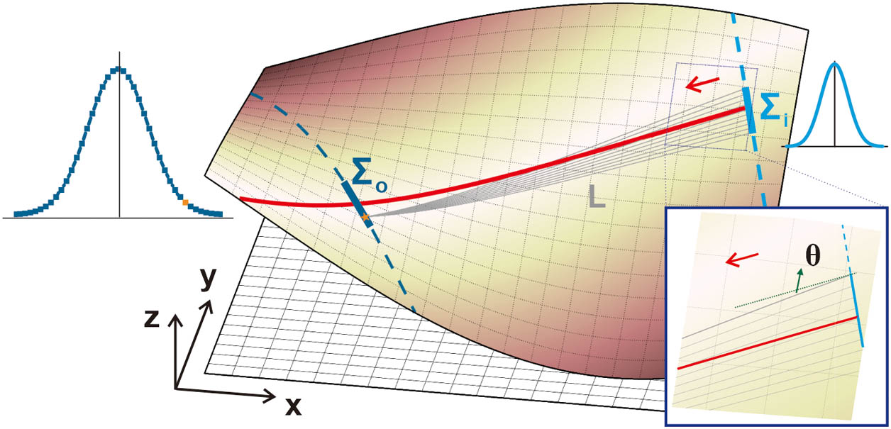
    Fig. 1. Schematic of a 2D curved surface generated from the planar Cartesian coordinates (x,y), here as an example with the height of the surface z=H(x,y)=sinxcosy. The red solid line denotes an arbitrary geodesic as the propagation axis of a light beam on this curved surface. Σi and Σo are the two geodesics locally vertical to the propagation axis as the input and output interfaces, respectively. The gray dark lines are the shortest geodesics from the points on Σi to the orange point on Σo, and one of the angles between these shortest geodesics and the propagation axis is denoted by θ in the inset figure.
    (a) (Left) Sketch of a Flamm’s paraboloid, and (right) the output-field intensity distribution at different propagation distance d for the cases of a well-collimated Gaussian beam launched from point A (the incident end) to points B1, B2, and B3 (different output ends) along the curve (ii). The curves (i)–(iv) with different colors on the surface show four typical geodesics along which a light beam propagates. (b) Magnitudes of the obliquity factor K between the input and output ends under different values of d=110 and 280 mm. (c) and (d) Changes of the beam width σ(d) of light along the geodesics (i) and (iii) in (a), respectively. The insets in (c) and (d) show the intensity evolution along the geodesics (i) and (iii), respectively, and the near-horizontal dot lines in (c) and (d) denote the changes of σ(d) in flat space. (e) and (f) The dependence of the output σ(d) on the initial σ0 along the four geodesics in (a) with the fixed value of d=220 mm, when the input end is locating differently at (e) r=200 mm and (f) r=300 mm. Other parameters are rs=20 mm, λ=7×10⁻⁵ m, r(Σi)=200 mm, σ0=10 mm.
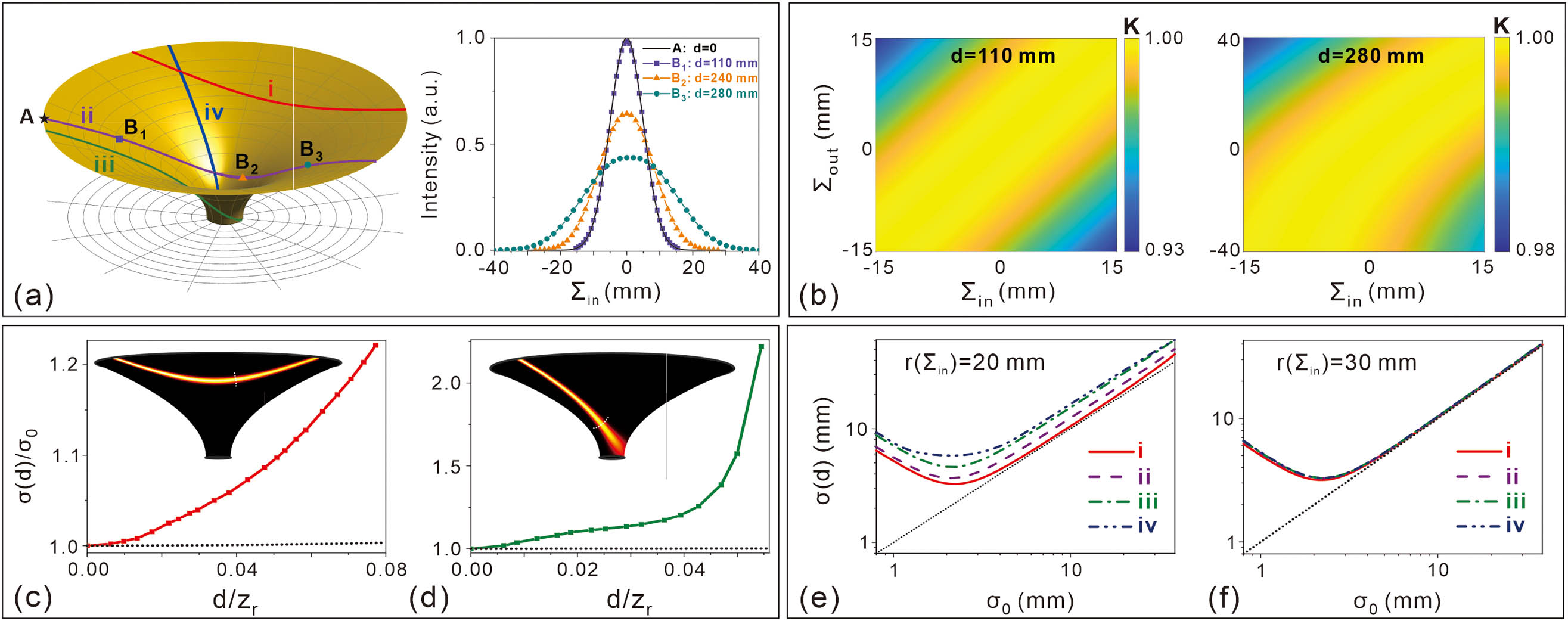
    Fig. 2. (a) (Left) Sketch of a Flamm’s paraboloid, and (right) the output-field intensity distribution at different propagation distance d for the cases of a well-collimated Gaussian beam launched from point A (the incident end) to points B1, B2, and B3 (different output ends) along the curve (ii). The curves (i)–(iv) with different colors on the surface show four typical geodesics along which a light beam propagates. (b) Magnitudes of the obliquity factor K between the input and output ends under different values of d=110 and 280 mm. (c) and (d) Changes of the beam width σ(d) of light along the geodesics (i) and (iii) in (a), respectively. The insets in (c) and (d) show the intensity evolution along the geodesics (i) and (iii), respectively, and the near-horizontal dot lines in (c) and (d) denote the changes of σ(d) in flat space. (e) and (f) The dependence of the output σ(d) on the initial σ0 along the four geodesics in (a) with the fixed value of d=220  mm, when the input end is locating differently at (e) r=200  mm and (f) r=300  mm. Other parameters are rs=20  mm, λ=7×10⁵  m, r(Σi)=200  mm, σ0=10  mm.
    (a) Sketch of two geodesics from a certain point (red) on the input to an arbitrary point (black cross or black asterisk) on the surface. (b) and (c) Intensity distributions (denoted by the common logarithm of intensity I=|Φo|2) in the green and blue regions of (a) are shown in (b) and (c), respectively, with magnitude being normalized by the maximal intensity of the incident light. Note that the intensity distribution in the gray region of (a) is not shown in (c) in case the intense field near the input end obscures the remaining region in (c). Other parameters are rs=15 mm, λ=1.5 cm, r(Σi)=150 mm, σ0=1 mm.
    Fig. 3. (a) Sketch of two geodesics from a certain point (red) on the input to an arbitrary point (black cross or black asterisk) on the surface. (b) and (c) Intensity distributions (denoted by the common logarithm of intensity I=|Φo|2) in the green and blue regions of (a) are shown in (b) and (c), respectively, with magnitude being normalized by the maximal intensity of the incident light. Note that the intensity distribution in the gray region of (a) is not shown in (c) in case the intense field near the input end obscures the remaining region in (c). Other parameters are rs=15  mm, λ=1.5  cm, r(Σi)=150  mm, σ0=1  mm.
    (a) Evolution of a light beam along a meridian of a hemisphere, with radius R, from the equator. The intensity profile of the light beam at the north pole along the geodesic (the blue line) is shown in the inset. (b) The intensity evolution of a light beam circling around a spherical surface along the direction (denoted by the orange arrow), starting from the geodesic (denoted by the blue solid line), which starts from r(Σi)=0.6R, φ(Σi)=π on the bottom projected plane. (c) Changes of beam width along the propagation on the spherical surface of (b). Other parameters are R=50 mm, λ=5×10⁻⁴ m, σ0=2 mm.
    Fig. 4. (a) Evolution of a light beam along a meridian of a hemisphere, with radius R, from the equator. The intensity profile of the light beam at the north pole along the geodesic (the blue line) is shown in the inset. (b) The intensity evolution of a light beam circling around a spherical surface along the direction (denoted by the orange arrow), starting from the geodesic (denoted by the blue solid line), which starts from r(Σi)=0.6R, φ(Σi)=π on the bottom projected plane. (c) Changes of beam width along the propagation on the spherical surface of (b). Other parameters are R=50  mm, λ=5×10⁴  m, σ0=2  mm.
    (a) Sketch of a Flamm’s paraboloid. (b1), (b2) Intensity distribution on the (b1) incident and (b2) opposite hemi-surface with wavelength λ=1.5×10⁻² m. These two subfigures are the same as Figs. 4(b) and 4(c). (c1), (c2) and (d1), (d2) Intensity of the field induced exclusively by (c1), (d1) CW and (c2), (d2) ACW geodesics along a certain latitude [white dashed lines in (b1) and (b2)] on the opposite hemi-surface (c1), (c2) and incident hemi-surface (d1), (d2). Due to symmetry, only a quarter of the surface is plotted, with φ labeled in (a). (c3), (d3) Intensity of the field after superimposing the complex amplitudes induced by CW and ACW geodesics. (e1), (e2) Intensity distribution of a light beam with the same parameters except for wavelength λ=1×10⁻⁵ m, which is therfore less divergent. Inset of (e2) is the zoom of the area in the blue dashed frame. (f1)–(f3) and (g1)–(g3) Intensity profiles along white dashed latitudes in (e1), (e2).
    Fig. 5. (a) Sketch of a Flamm’s paraboloid. (b1), (b2) Intensity distribution on the (b1) incident and (b2) opposite hemi-surface with wavelength λ=1.5×10²  m. These two subfigures are the same as Figs. 4(b) and 4(c). (c1), (c2) and (d1), (d2) Intensity of the field induced exclusively by (c1), (d1) CW and (c2), (d2) ACW geodesics along a certain latitude [white dashed lines in (b1) and (b2)] on the opposite hemi-surface (c1), (c2) and incident hemi-surface (d1), (d2). Due to symmetry, only a quarter of the surface is plotted, with φ labeled in (a). (c3), (d3) Intensity of the field after superimposing the complex amplitudes induced by CW and ACW geodesics. (e1), (e2) Intensity distribution of a light beam with the same parameters except for wavelength λ=1×10⁵  m, which is therfore less divergent. Inset of (e2) is the zoom of the area in the blue dashed frame. (f1)–(f3) and (g1)–(g3) Intensity profiles along white dashed latitudes in (e1), (e2).
    Chenni Xu, Li-Gang Wang. Theory of light propagation in arbitrary two-dimensional curved space[J]. Photonics Research, 2021, 9(12): 2486
    Download Citation