Theory of light propagation in arbitrary two-dimensional curved space

Chenni Xu; Li-Gang Wang

doi:10.1364/PRJ.435993

Abstract

As an analog model of general relativity, optics on some two-dimensional (2D) curved surfaces has received increasing attention in the past decade. Here, in light of the Huygens–Fresnel principle, we propose a theoretical frame to study light propagation along arbitrary geodesics on any 2D curved surfaces. This theory not only enables us to solve the enigma of “infinite intensity” that existed previously at artificial singularities on surfaces of revolution but also makes it possible to study light propagation on arbitrary 2D curved surfaces. Based on this theory, we investigate the effects of light propagation on a typical surface of revolution, Flamm’s paraboloid, as an example, from which one can understand the behavior of light in the curved geometry of Schwarzschild black holes. Our theory provides a convenient and powerful tool for investigations of radiation in curved space.

1. INTRODUCTION

In general relativity (GR), spacetime is distorted in the vicinity of massive celestial bodies. Dynamics of electromagnetic (EM) waves in the context of strong gravitational fields has attracted increasing attention, ranging from wave optics [1] to gravitational lensing [2] and scattering theory [3], as well as photon rings [4], which are predicted to be ensconced in the shadow of the M87* black hole image recently published by EHT Collaboration [5]. Despite the flourishing astrophysical explorations, investigations from the perspective of optics are still rare. Because of feeble gravitational effects, measurements and verification of GR phenomena are difficult to perform unless in an astronomical scale. Therefore, researchers have proposed various analog models to study GR phenomena using tabletop equipment in laboratories [6], such as observation of spontaneous Hawking radiation in a flowing Bose–Einstein condensate [7], emulation of Schwarzschild precession with a gradient index lens [8], and mimicking gravitational lensing by a microstructured optical waveguide [9]. Another analog model is to abandon one spatial dimension and fix the time coordinate of the four-dimensional (4D) curved spacetime. In this manner, the remaining 2D spatial metric tensor can be depicted as a 2D curved surface embedded in 3D space, and the interplay between EM waves and spatial curvature can be revealed by investigating light propagation on such appropriately fabricated surfaces. Ever since this notion was put forward by Batz and Peschel [10] in 2008, various optical phenomena have been reported both theoretically [10 –18] and experimentally [19 –23]. Besides optics and photonics, similar studies on curved surfaces have also been extended to surface plasmon polaritons [24], acoustic topological insulators [25], and quantum particles [26].

The theory of light propagation in 2D curved space was initiated by Batz and Peschel [10], by obtaining a nonlinear Schrödinger equation on surfaces of revolution (SORs) with constant Gaussian curvature. Owing to the rotational symmetry of SORs, the curvilinear coordinates on surfaces are conveniently taken along longitudes and latitudes. This paradigm ingeniously simplifies the calculation to a great extent. However, the solution applies exclusively to propagation along the longitudinal direction, which is special among innumerable geodesics. Indeed, considering light propagation along non-longitudinal directions is more challenging, not only because of the tedious calculation of analytically solving the covariant wave equation but also the ambiguous physical images that are beyond intuitive imagination. Due to the rotational symmetry of SORs, a light beam launched tangent to a longitude recognizes an axisymmetric distribution of spatial curvature, which guarantees its propagation right along the very longitude. However, such axisymmetry does not hold true for light beams with other initial directions, whose trajectories will therefore be bent somehow. Intriguing questions naturally arise; for instance, which pathway would the light beam take and how would the curvature of the surface affect its divergence? It has also been revealed in prior studies [10,15,17,20] that the existing method for calculating light fields on closed SORs collapsed at artificial singularities (such as both the north and south poles on spherical surfaces), leading to an artificial “infinite intensity” thereat.

In this paper, we propose an alternative approach to study light propagation along arbitrary geodesics on any curved surfaces, in light of the Huygens–Fresnel principle. We assume the light wave propagates along the geodesic, the natural path of its ray counterpart in curved space. This approach not only figures out the problems mentioned above but also in a manner that refrains from using complicated mathematics. With this approach, we take a Flamm’s paraboloid, which is the 2D correspondence of the Schwarzschild metric, as an example, and we demonstrate the behaviors of both collimated and highly divergent light in such curved space. We then figure out the remaining enigma of artificial singularities in the previous method and suggest some possible schemes for experimental verification.

Sign up for Photonics Research TOC. Get the latest issue of Photonics Research delivered right to you！Sign up now

2. RESULTS AND DISCUSSION

A. Basic Theory

Consider an arbitrary 2D curved surface that can be fabricated by deforming a plane. The points on an arbitrary curved surface can be expressed by the 3D Cartesian coordinates as $[x, y, z = H (x, y)]$ , with $x$ , $y$ being the planar Cartesian coordinates and an arbitrary function $H$ marking the height difference between the curved surface and the $x y$ plane, as is sketched in Fig. 1. The corresponding metric of the curved surface is $d s^{2} = g_{i j} d x^{i} d x^{j} = [1 + {(\frac{\partial H}{\partial x})}^{2}] d x^{2} + [1 + {(\frac{\partial H}{\partial y})}^{2}] d y^{2} + 2 \frac{\partial H}{\partial x} \frac{\partial H}{\partial y} d x d y,$ (1)where the third term indicates that the coordinate system we choose to parametrize the surface is not orthogonal on the curved surface. On curved surfaces, light rays propagate along the so-called geodesics, which are the counterparts of the straight lines in flat space. The geodesic equation is given by $\frac{d^{2} x^{σ}}{d s^{2}} + Γ_{μ ν}^{σ} \frac{d x^{μ}}{d s} \frac{d x^{ν}}{d s} = 0$ , where $Γ_{μ ν}^{σ} = \frac{1}{2} g^{σ ρ} (\frac{\partial g_{ρ μ}}{\partial x^{ν}} + \frac{\partial g_{ρ ν}}{\partial x^{μ}} - \frac{\partial g_{μ ν}}{\partial x^{ρ}})$ are Christoffel connections, $g^{σ ρ}$ are the elements of the inverse of the metric tensor $g$ , and Einstein summation convention is applied, with $x^{σ}, x^{μ}, x^{ν}$ running through $x$ , $y$ . Therefore, one can track a light ray on a curved surface by solving the following equations: $\frac{d^{2} x}{d s^{2}} + Γ_{x x}^{x} {(\frac{d x}{d s})}^{2} + Γ_{y y}^{x} {(\frac{d y}{d s})}^{2} + 2 Γ_{x y}^{x} \frac{d x}{d x} \frac{d y}{d s} = 0,$ (2) $\frac{d^{2} y}{d s^{2}} + Γ_{x x}^{y} {(\frac{d x}{d s})}^{2} + Γ_{y y}^{y} {(\frac{d y}{d s})}^{2} + 2 Γ_{x y}^{y} \frac{d x}{d s} \frac{d y}{d s} = 0 .$ (3)Generally, it is difficult to acquire the analytical solution to this equation set, unless some extra properties of surfaces, such as symmetries, are present. Usually numerical methods, such as the Runge–Kutta method, can be used to solve the above equations as long as the step length meets the accuracy requirements. We would like to make a remark here that in this work, we consider exclusively a spatial metric. This reduction is justified if Eq. (1) is the “Fermat metric” (aka “optical metric”; see Ref. [27] and references therein) of a 4D spacetime metric, where the projection of a 4D null geodesic in its spatial section is exactly the solution of Eqs. (2) and (3).

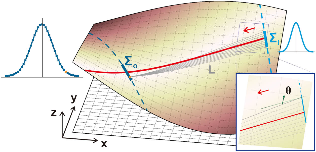
Figure 1.Schematic of a 2D curved surface generated from the planar Cartesian coordinates $(x, y)$ , here as an example with the height of the surface $z = H (x, y) = \sin x \cos y$ . The red solid line denotes an arbitrary geodesic as the propagation axis of a light beam on this curved surface. $Σ_{i}$ and $Σ_{o}$ are the two geodesics locally vertical to the propagation axis as the input and output interfaces, respectively. The gray dark lines are the shortest geodesics from the points on $Σ_{i}$ to the orange point on $Σ_{o}$ , and one of the angles between these shortest geodesics and the propagation axis is denoted by $θ$ in the inset figure.

Now let us consider the propagation of light on curved surfaces. First, we build up the coordinates on a curved surface, as is shown in Fig. 1. The optical propagation axis of a light beam is taken along the arbitrary geodesic that we are interested in, e.g., the red line on the surface. Vertical to the optical propagation axis, the input and output interfaces are taken along the orthogonal geodesics, respectively, denoted by $Σ_{i}$ and $Σ_{o}$ on that surface. In light of the Huygens–Fresnel principle, each point $S_{i}$ on the input interface $Σ_{i}$ is a source of secondary spherical wavelet. The secondary wavelets emanating from different points on the initial interface interfere mutually; the superposition forms the far-field wavefront at $P_{o}$ on the output interface $Σ_{o}$ . Put mathematically, the complex amplitude at $P_{o}$ on $Σ_{o}$ is described as $Φ_{o} (P_{o}) = \sqrt{\frac{1}{i λ}} \int_{Σ_{i}} Φ_{i} (S_{i}) \frac{e^{i k L (S_{i}, P_{o})}}{L (S_{i}, P_{o})} K (S_{i}, P_{o}) d l,$ (4)where $Φ_{i} (S_{i})$ and $Φ_{o} (P_{o})$ are, respectively, the incident and output complex fields at the input and output ends, $k = 2 π / λ$ is the wavenumber with wavelength $λ$ , and $d l$ denotes the primary wave source on the incident end $Σ_{i}$ , which now is essentially 1D. Here, $K = \cos θ$ is the obliquity factor, with $θ$ being the angle between the propagation axis and the geodesic connecting any input point $S_{i}$ on $Σ_{i}$ and the output point $P_{o}$ on $Σ_{o}$ , as is shown in the inset of Fig. 1. Figure 2(b) shows that this obliquity factor can be reasonably taken as $1$ when the propagation distance $d$ is 1 order of magnitude larger than the transverse dimension. Here, we emphasize again that both the incident and output ends, $Σ_{i}$ and $Σ_{o}$ , should be taken along the geodesics, which are locally orthogonal to the propagation optical axis, and thus the points on $Σ_{i}$ and $Σ_{o}$ are $S_{i} = (x, y, z)$ and $P_{o} = (x^{'}, y^{'}, z^{'})$ , obeying Eqs. (2) and (3). The function $L (S_{i}, P_{o})$ represents the eikonal function, which is essentially the length of the geodesic connecting $S_{i}$ on $Σ_{i}$ and $P_{o}$ on $Σ_{o}$ , obtained by $L = \int d s$ . Technically, except for a few special surfaces, the analytical expression of $L$ is scarcely available, leading to the difficulty in the integral in Eq. (4). Therefore, in practice, for a certain point $P_{o}$ on $Σ_{o}$ , we also calculate the geodesic lengths directly, according to Eqs. (2) and (3), connecting $P_{o}$ and hundreds of discrete points $S_{i}$ on $Σ_{i}$ , which are deviated from the optical propagation axis as shown in Fig. 1. Thus one can obtain the exact field distribution of light along $Σ_{o}$ .

Figure 2.(a) (Left) Sketch of a Flamm’s paraboloid, and (right) the output-field intensity distribution at different propagation distance $d$ for the cases of a well-collimated Gaussian beam launched from point A (the incident end) to points $B_{1}$ , $B_{2}$ , and $B_{3}$ (different output ends) along the curve (ii). The curves (i)–(iv) with different colors on the surface show four typical geodesics along which a light beam propagates. (b) Magnitudes of the obliquity factor $K$ between the input and output ends under different values of $d = 110$ and 280 mm. (c) and (d) Changes of the beam width $σ (d)$ of light along the geodesics (i) and (iii) in (a), respectively. The insets in (c) and (d) show the intensity evolution along the geodesics (i) and (iii), respectively, and the near-horizontal dot lines in (c) and (d) denote the changes of $σ (d)$ in flat space. (e) and (f) The dependence of the output $σ (d)$ on the initial $σ_{0}$ along the four geodesics in (a) with the fixed value of $d = 220 mm$ , when the input end is locating differently at (e) $r = 200 mm$ and (f) $r = 300 mm$ . Other parameters are $r_{s} = 20 mm$ , $λ = 7 \times 10^{- 5} m$ , $r (Σ_{i}) = 200 mm$ , $σ_{0} = 10 mm$ .

In practice, the rotational symmetry exists extensively in many celestial systems. Here we consider a special family of curved surfaces with rotational symmetry, universally known as SORs, whose metrics can be generally expressed as $d s^{2} = [1 + {(\frac{d H}{d r})}^{2}] d r^{2} + r^{2} d φ^{2}$ in a polar coordinate system for convenience. Thanks to the orthogonality of the coordinates as well as the rotational symmetry, now one is able to solve Eqs. (2) and (3) analytically (for mathematical details, see Appendix A): $d φ = \pm \frac{κ}{r \sqrt{r^{2} - κ^{2}}} \sqrt{1 + {(\frac{d H}{d r})}^{2}} d r,$ (5)where $κ = r_{initial}^{2} {(\frac{d φ}{d s})}_{initial}$ is a constant determined by initial conditions, and the sign of $\pm$ corresponds to two different trajectories according to the sign of the initial condition $\frac{d r}{d s}$ .

B. Light Propagation on Flamm’s Paraboloids

Next we will use the above approach to consider the light propagation on a specific SOR, the Flamm’s paraboloid, as is shown in Fig. 2(a). This interesting surface reveals the spatial curvature in the vicinity of a Schwarzschild black hole [28]. As known, the gravitational field outside the Schwarzschild radius $r_{s}$ of an uncharged irrotational spherical mass is described by the Schwarzschild metric: $d s^{2} = - (1 - \frac{r_{s}}{r}) c^{2} d t^{2} + {(1 - \frac{r_{s}}{r})}^{- 1} d r^{2} + r^{2} d ψ^{2} + r^{2} \sin^{2} ψ d φ^{2} .$ (6)With its spherical symmetry, the equatorial slice is taken (i.e., $ψ = π / 2$ ) without loss of generality, and the remnant of the spatial part of Eq. (6) establishes an SOR with $H (r) = \pm 2 \sqrt{r_{s} (r - r_{s})}$ for $r > r_{s}$ . As shown in Fig. 2(a), first we consider the propagation of a well-collimated Gaussian wave packet launched along four different geodesics. The Gaussian profile is well maintained at an arbitrary output end when the beam is a little bit away from the event horizon of the black hole. For example, when the beam propagates along the curve (ii) (the purple curve), the beam width changes little from $A$ to $B_{1}$ since the light is far away from the black hole ( $r ≫ r_{s}$ ), while it increases fast as the light approaches the black hole, such as near the points $B_{2}$ and $B_{3}$ . The intensity profiles at these points are shown in the right side of Fig. 2(a). In this situation, we can define the beam width $σ$ of light as the full width at its half maximum of the intensity profile and track its evolution along the propagation. The changes of the beam width along the red and green geodesics in Fig. 2(a) are demonstrated in Figs. 2(c) and 2(d), respectively, along with their intensity evolution in the corresponding inset figures. The propagation distance $d$ along the propagation axis is normalized by the Rayleigh distance $z_{r}$ of light in flat space. It is seen that the light beams in both of these cases diverge rapidly even within a short distance compared to the cases in flat space. This tells us that the divergence of light beams on such a curved surface is greatly amplified due to the large spatial curvature generated from the strong gravitational field near the black hole. The diverging nature of light beams on Flamm’s paraboloid is further revealed in Figs. 2(e) and 2(f), where the variation of $σ (d)$ at a certain output end versus the initial beam width $σ_{0}$ along the four geodesics in Fig. 2(a) is illustrated. We can see that the Gaussian beams with small $σ_{0}$ are subject to strong divergence, under the same $d$ , due to the experience of the strong spatial curvature, and the turning points in these four cases are slightly different. These effects are actually related to the strength of negative spatial curvature [10,14].

Now we consider the propagation of a very narrow light beam with a large divergent angle launched directly toward the black hole, along the geodesic (iv) in Fig. 2(a). This is usually similar to the situation that a point-like light source is far away from a black hole. The beam is so divergent that instead of being entirely captured, only the central portion is absorbed by the event horizon, while the periphery grazes the black hole and escapes. As a result, signals can be detected at the opposite side of the light source (i.e., the forward scattering), or even be detected at the same side of the light source (i.e., the backward scattering). In practice, we calculate the distribution of the light field on the entire surface of Flamm’s paraboloid, rather than taking a specific far-field output end as we did above. Interestingly, there are always two possible geodesics from a certain point on the input interface to an arbitrary point on such Flamm’s paraboloid surface of the black hole. As an example, in Fig. 3(a), we can see that light rays can travel clockwise and anticlockwise along two different geodesics, respectively, to reach the cross and/or asterisk points in the forward and/or backward directions. The interplay of these two branches of light rays may lead to interference fringes on the forward hemi-surface, as is clearly revealed in Fig. 3(b). Such behaviors are similar to the interference characteristics shown in a recent work by Nambu et al. [1]. Furthermore, some portions of light rays may even return as the backward scattering, via the backward geodesics after circling around the black hole, to the vicinity of the incident source, resulting in the complicated interference patterns in Fig. 3(c). We believe such forward-scattering and backward-scattering phenomena, in spite of its feebleness, could possibly be used to obtain the structural information of black holes and detect the gravitational effects of invisible and small black holes. More detailed properties of the forward- and backward-scattering effects for light near a black hole will be further explored elsewhere. Indeed, the interaction between two branches of rays also exists in the collimated light beams investigated in the above, yet one branch dominates, and consequently no interference can be observed (see Appendix B).

Figure 3.(a) Sketch of two geodesics from a certain point (red) on the input to an arbitrary point (black cross or black asterisk) on the surface. (b) and (c) Intensity distributions (denoted by the common logarithm of intensity $I = {| Φ_{o} |}^{2}$ ) in the green and blue regions of (a) are shown in (b) and (c), respectively, with magnitude being normalized by the maximal intensity of the incident light. Note that the intensity distribution in the gray region of (a) is not shown in (c) in case the intense field near the input end obscures the remaining region in (c). Other parameters are $r_{s} = 15 mm$ , $λ = 1.5 cm$ , $r (Σ_{i}) = 150 mm$ , $σ_{0} = 1 mm$ .

C. Deciphering the Leftover Singularity Puzzle

In Ref. [10], an ingenious expression about the propagation of a light beam on the special SORs with constant Gaussian curvature is analytically given by solving the covariant Helmholtz equation in the longitude–latitude coordinate system under paraxial approximation. Taking the hemispherical surface in Fig. 4(a) as an example, the longitudinal coordinate $u$ along the longitudinal arc direction has the range of $u \in [0, π R / 2]$ , with $R$ being the radius of the hemisphere, while the latitudinal coordinate $v$ , being the rotational angle, is within the range $[0, 2 π]$ . The arc length of latitudes is thus $2 π R \cos (u / R)$ , which varies with $u$ and vanishes at the north pole $u = π R / 2$ , resulting in a mathematical singularity. The intensity evolution of a Gaussian beam propagating along the meridian and starting from the equator follows $I (u, v) = \frac{1}{\cos (\frac{u}{R}) {[1 + R^{2} \tan^{2} (\frac{u}{R}) / z_{r}^{2}]}^{1 / 2}} \times \exp [- \frac{k z_{r} R^{2} v^{2}}{R^{2} \tan^{2} (\frac{u}{R}) + z_{r}^{2}}],$ (7)where $z_{r} = k σ_{0}^{2} / 2$ is the Rayleigh distance in flat space, and accordingly the beam width obeys $σ (u) = σ_{0} \sqrt{\cos^{2} (\frac{u}{R}) + \frac{R^{2}}{z_{r}^{2}} \sin^{2} (\frac{u}{R})},$ (8)where $σ_{0}$ is the initial beam width (for the detailed derivation, see Appendix C). Apparently the intensity is infinite at $u = π R / 2$ , yet the beam width is not vanishing at the singularity. Such singularity will not occur when the light beam propagates along the equator, which, however, should be exactly identical to the propagation along a meridian, owing to the perfect symmetry of a sphere. Clearly, such singular behaviors along a meridian are artificial.

Figure 4.(a) Evolution of a light beam along a meridian of a hemisphere, with radius $R$ , from the equator. The intensity profile of the light beam at the north pole along the geodesic (the blue line) is shown in the inset. (b) The intensity evolution of a light beam circling around a spherical surface along the direction (denoted by the orange arrow), starting from the geodesic (denoted by the blue solid line), which starts from $r (Σ_{i}) = 0.6 R$ , $φ (Σ_{i}) = π$ on the bottom projected plane. (c) Changes of beam width along the propagation on the spherical surface of (b). Other parameters are $R = 50 mm$ , $λ = 5 \times 10^{- 4} m$ , $σ_{0} = 2 mm$ .

Fundamentally, these puzzles are consequences of mischoice of the far-field output interface and can be well solved by the method mentioned in this work. In the longitude–latitude coordinate system, both the incident and far-field interfaces are supposed to be taken along the latitudinal lines, which are actually not geodesics (except the equator). In practice, when an observer stands on the curved surface, the coordinates should be taken locally along the two orthogonal geodesics. In this situation, the propagation of a light beam is illustrated in Fig. 4(a). In particular, on the north pole, the geodesic perpendicular to the propagation axis is marked by the blue bold line, and thus the north pole is naturally a regular point instead of an artificial singularity. Furthermore, we also inspect the propagation of a light beam circling a sphere in Fig. 4(b) and find that the evolution of the beam width oscillates after each half circumference on the spherical surface. This interesting property was discovered under the condition that the propagation is along the equator via the coordinate transformation [10]. By our method, this periodic oscillation of the beam width can also be obtained when the incident Gaussian beam starts from arbitrary positions on a sphere, which is unavailable in the previous method. These results not only solve the artificial singularity enigma but are also more pragmatic in real experiments, since it is more appropriate to take an arbitrary geodesic as the incident interface when a laser beam is coupled onto a curved surface.

D. Possible Experimental Schemes

Our theory can be experimentally implemented both macroscopically and microscopically. In pioneering experiments, constraining light propagation on curved surfaces was realized either by total internal reflection in curved crown glass [19 –21] or by a thin liquid waveguide covered on a 3D solid object [19,20]. The 3D objects with prescribed shapes can be fabricated by state-of-the-art technologies, such as high-precision diamond turning for macroscopic structures [19] and the Nanoscribe 3D laser lithography technique [22,29] in nanometric scale. Very recently, an intriguing work [30] demonstrates light propagation on thin curved soap membranes (see its supplementary video 3). This scheme provides a promising novel platform, especially when the varying thickness of the membrane, acting as an effective refractive index, could be an extra dimension for modulation. Moreover, it is proved that a curved surface of revolution is equivalent to a plane with azimuthally symmetric distribution of refractive index [31]. Therefore, an alternative pathway is to fabricate the predesigned refractive index profile on a planar surface, by, e.g., a microsphere-embedded variable-thickness polymethyl methacrylate waveguide [9,32], or through the optically induced giant Kerr effect in liquid crystal [33], with its landscape being provided by a spatial light modulator working in reflection.

3. CONCLUSION

In conclusion, we develop heuristics to study the propagation of light in 2D curved space, founded on the Huygens–Fresnel principle. This method is feasible when the direction of light propagation is along arbitrary geodesics on any curved surface. By this method, we study the behaviors of light beams on a Flamm’s paraboloid, which is the 2D correspondence of spatial curvature outside a Schwarzschild black hole. We investigate the evolution of Gaussian wave packets propagating along different geodesics and reveal the diverging nature of light on such curved surfaces. We also illustrate the interference patterns induced by highly divergent light sources. Finally, we point out that this method works out the remaining puzzles about the coordinate singularities in the previous theory. Our work provides a powerful tool and refreshing insights that greatly broaden the possibilities of investigations about light propagation in curved space. Exotic geodesics [34] could be used to realize lights with special properties. With the help of the proposed method, further studies could be extended to other optical effects, such as spectral properties [14,15], phase information [17], the Hanbury Brown and Twiss effect [20], geodesic lens [35], the Talbot effect [36], and acceleration radiation [37]. Moreover, the investigations about optics on Flamm’s paraboloids open up a new perspective on the radiations in the vicinity of Schwarzschild black holes and contribute to the interdisciplinary explorations of cosmology and optics.

APPENDIX A: DERIVATION OF EQ.?(5)

d s^{2} = [1 + {(\frac{d H}{d r})}^{2}] d r^{2} + r^{2} d φ^{2} .

APPENDIX B: SUPERPOSITION OF CLOCKWISE AND ANTICLOCKWISE GEODESICS

Figure 5.(a) Sketch of a Flamm’s paraboloid. (b1), (b2) Intensity distribution on the (b1) incident and (b2) opposite hemi-surface with wavelength $λ = 1.5 \times 10^{- 2} m$ . These two subfigures are the same as Figs. 4(b) and 4(c). (c1), (c2) and (d1), (d2) Intensity of the field induced exclusively by (c1), (d1) CW and (c2), (d2) ACW geodesics along a certain latitude [white dashed lines in (b1) and (b2)] on the opposite hemi-surface (c1), (c2) and incident hemi-surface (d1), (d2). Due to symmetry, only a quarter of the surface is plotted, with $φ$ labeled in (a). (c3), (d3) Intensity of the field after superimposing the complex amplitudes induced by CW and ACW geodesics. (e1), (e2) Intensity distribution of a light beam with the same parameters except for wavelength $λ = 1 \times 10^{- 5} m$ , which is therfore less divergent. Inset of (e2) is the zoom of the area in the blue dashed frame. (f1)–(f3) and (g1)–(g3) Intensity profiles along white dashed latitudes in (e1), (e2).

APPENDIX C: DERIVATION OF EQS.?(7) AND (8)

\frac{1}{\sqrt{g}} \partial_{i} (\sqrt{g} g^{i j} \partial_{j} Φ) + k^{2} Φ = 0,

Φ (u, v) = {[\cos (\frac{u}{R})]}^{- \frac{1}{2}} Ψ (u, v)

ϕ (u, v) = \exp [i α (u) + \frac{i k v^{2}}{2 β (u)}],

References

[1] Y. Nambu, S. Noda, Y. Sakai. Wave optics in spacetimes with compact gravitating object. Phys. Rev. D, 100, 064037(2019).

[2] S. E. Gralla, A. Lupsasca. Lensing by Kerr black holes. Phys. Rev. D, 101, 044031(2020).

[3] J. A. H. Futterman, F. A. Handler, R. A. Matzner. Scattering from Black Holes(2009).

[4] M. D. Johnson, A. Lupsasca, A. Strominger, G. N. Wong, S. Hadar, D. Kapec, R. Narayan, A. Chael, C. F. Gammie, P. Galison, D. C. M. Palumbo, S. S. Doeleman, L. Blackburn, M. Wielgus, D. W. Pesce, J. R. Farah, J. M. Moran. Universal interferometric signatures of a black hole’s photon ring. Sci. Adv., 6, eaaz1310(2020).

[5] The Event. First M87 event horizon telescope results. I. The shadow of the supermassive black hole. Astrophys. J. Lett., 875, L1(2019).

[6] D. Faccio, F. Belgiorno, S. Cacciatori, V. Gorini, S. Liberati, U. Moschella. Analogue Gravity Phenomenology: Analogue Spacetimes and Horizons, from Theory to Experiment(2013).

[7] J. R. M. de Nova, K. Golubkov, V. I. Kolobov, J. Steinhauer. Observation of thermal Hawking radiation and its temperature in an analogue black hole. Nature, 569, 688-691(2019).

[8] W. Xiao, S. Tao, H. Chen. Mimicking the gravitational effect with gradient index lenses in geometrical optics. Photon. Res., 9, 1197-1203(2021).

[9] C. Sheng, H. Liu, S. N. Zhu, D. A. Genov. Trapping light by mimicking gravitational lensing. Nat. Photonics, 7, 902-906(2013).

[10] S. Batz, U. Peschel. Linear and nonlinear optics in curved space. Phys. Rev. A, 78, 043821(2008).

[11] S. Batz, U. Peschel. Solitons in curved space of constant curvature. Phys. Rev. A, 81, 053806(2010).

[12] R. Bekenstein, J. Nemirovsky, I. Kaminer, M. Segev. Shape-preserving accelerating electromagnetic wave packets in curved space. Phys. Rev. X, 4, 011038(2014).

[13] E. Lustig, M.-I. Cohen, R. Bekenstein, G. Harari, M. A. Bandres, M. Segev. Curved-space topological phases in photonic lattices. Phys. Rev. A, 96, 041804(2017).

[14] C. Xu, A. Abbas, L.-G. Wang, S.-Y. Zhu, M. S. Zubairy. Wolf effect of partially coherent light fields in two-dimensional curved space. Phys. Rev. A, 97, 063827(2018).

[15] C. Xu, A. Abbas, L.-G. Wang. Generalization of Wolf effect of light on arbitrary two-dimensional surface of revolution. Opt. Express, 26, 33263-33277(2018).

[16] D. Wang, C. Liu, H. Liu, J. Han, S. Zhang. Wave dynamics on toroidal surface. Opt. Express, 26, 17820-17829(2018).

[17] C. Xu, L.-G. Wang. Gouy and spatial-curvature-induced phase shifts of light in two-dimensional curved space. New J. Phys., 21, 113013(2019).

[18] Z. Shao, Z. Wang. Propagation and transformation of a light beam on a curved surface. Opt. Express, 29, 8626-8634(2021).

[19] V. H. Schultheiss, S. Batz, A. Szameit, F. Dreisow, S. Nolte, A. Tünnermann, S. Longhi, U. Peschel. Optics in curved space. Phys. Rev. Lett., 105, 143901(2010).

[20] V. H. Schultheiss, S. Batz, U. Peschel. Hanbury Brown and Twiss measurements in curved space. Nat. Photonics, 10, 106-110(2016).

[21] A. Patsyk, M. A. Bandres, R. Bekenstein, M. Segev. Observation of accelerating wave packets in curved space. Phys. Rev. X, 8, 011001(2018).

[22] R. Bekenstein, Y. Kabessa, Y. Sharabi, O. Tal, N. Engheta, G. Eisenstein, A. J. Agranat, M. Segev. Control of light by curved space in nanophotonic structures. Nat. Photonics, 11, 664-670(2017).

[23] J. Zhu, Y. Liu, Z. Liang, T. Chen, J. Li. Elastic waves in curved space: mimicking a wormhole. Phys. Rev. Lett., 121, 234301(2018).

[24] A. Libster-Hershko, R. Shiloh, A. Arie. Surface plasmon polaritons on curved surfaces. Optica, 6, 115-118(2019).

[25] H. W. Wu, J. Q. Quan, Y. K. Liu, Y. Pan, Z. Q. Sheng, L. W. Jing. Observation of protected localized states induced by curved space in acoustic topological insulators(2021).

[26] G. D. Valle, M. Savoini, M. Ornigotti, P. Laporta, V. Foglietti, M. Finazzi, L. Duò, S. Longhi. Experimental observation of a photon bouncing ball. Phys. Rev. Lett., 102, 180402(2009).

[27] V. Perlick. Gravitational lensing from a spacetime perspective. Living Rev. Relativ., 7, 9-117(2004).

[28] C. W. Misner, K. S. Thorne, J. A. Wheeler. Gravitation(1973).

[29] S. Maruo, O. Nakamura, S. Kawata. Three-dimensional microfabrication with two-photon-absorbed photopolymerization. Opt. Lett., 22, 132-134(1997).

[30] A. Patsyk, U. Sivan, M. Segev, M. A. Bandres. Observation of branched flow of light. Nature, 583, 60-66(2020).

[31] C. Xu, I. Dana, L.-G. Wang, P. Sebbah. Light chaotic dynamics in the transformation from curved to flat surfaces(2021).

[32] C. Sheng, R. Bekenstein, H. Liu, S. Zhu, M. Segev. Wavefront shaping through emulated curved space in waveguide settings. Nat. Commun., 7, 10747(2016).

[33] I. C. Khoo. Extreme nonlinear optics of nematic liquid crystals. J. Opt. Soc. Am. B, 28, A45-A55(2011).

[34] A. L. Besse. Manifolds All of Whose Geodesics Are Closed(1978).

[35] L. Xu, X. Wang, T. Tyc, C. Sheng, S. Zhu, H. Liu, H. Chen. Light rays and waves on geodesic lenses. Photon. Res., 7, 1266-1272(2019).

[36] L. A. Hall, M. Yessenov, S. A. Ponomarenko, A. F. Abouraddy. The space–time Talbot effect. APL Photon., 6, 056105(2021).

[37] M. O. Scully, S. Fulling, D. M. Lee, D. N. Page, W. P. Schleich, A. A. Svidzinsky. Quantum optics approach to radiation from atoms falling into a black hole. Proc. Nat. Acad. Sci. USA, 115, 8131-8136(2018).