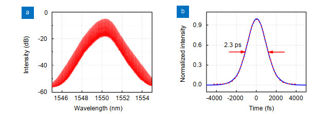
Fig. 1. The 10 GHz OFC and a 2.3-ps pulse generated from a mode-locked laser with (a) OFC spectrum, and (b) reconstructed temporal pulse profile (blue solid curve) and Gaussian fitting curve (red dotted curve).

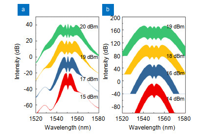
Fig. 2. Optical spectra after propagation in 500 m HNLF. (a) The experimental results when the input optical power into the HNLF is 15 dBm, 17 dBm, 19 dBm, 20 dBm, respectively. (b) The simulation results when the input optical power is 14 dBm, 16 dBm, 18 dBm, 19 dBm, respectively.

Fig. 3. (a) RF spectrum from the broadened frequency comb at 20 dBm pump power (RBW=200 kHz and VBW=50 kHz). (b) Reconstructed temporal pulse profile with a FWHM duration of 291 fs after transmitting a 4 m SMF at 20 dBm pump power (blue solid curve) and Gaussian fitting curve (red dotted curve).

Fig. 4. Optical spectra of the generated flat-topped OFC. (a) The 10 GHz repetition rate at 26.5 dBm pump power. (b) The 18.5 GHz repetition rate at 25.5 dBm pump power.

Fig. 5. (a) Experimental supercontinuum spectra designed to produce a dispersive wave centered around 1310 nm. (b) RF spectra from the generated 1310 nm dispersion wave at 32 dBm pump power (RBW=200 kHz and VBW=50 kHz).

Fig. 6. The calculated dispersions of the fibers with different sizes. Insets, scanning electron microscope images of the fibers with the diameters of 3.7 μm, 3.3 μm and 3.1 μm, respectively.

Fig. 7. (a) Optical spectra with a dispersive wave centered around 1310 nm from a fluorotellurite fiber under different launched powers of the femtosecond laser. (b) Optical spectra with tunable dispersive waves ranging from 1150 nm to 1310 nm from fluorotellurite fibers 1, 2, 3 with ZDWs at 1358 nm, 1409 nm and 1452 nm, respectively.

Fig. 8. (a) The simulated and measured SC from the fluorotellurite fiber with the ZDW of 1452 nm and the peak pump power of 387 W. (b) RF spectrum from the generated 1310 nm dispersion wave in the fluorotellurite fiber (RBW=200 kHz and VBW=50 kHz).