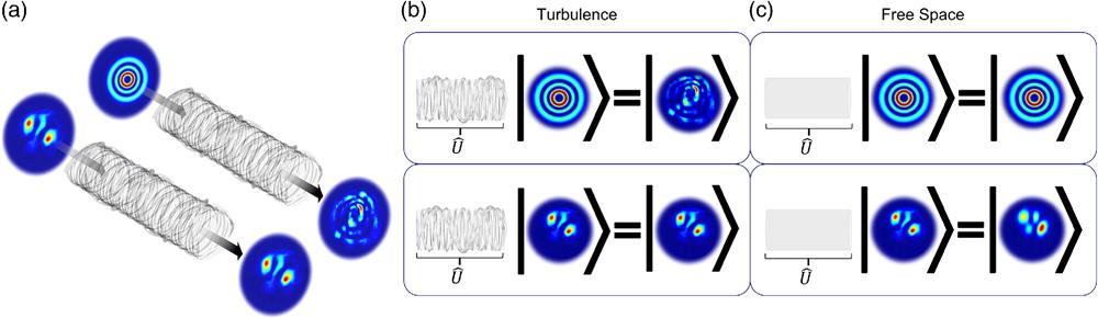
Fig. 1. Propagation through turbulence: (a) most common forms of structured light (such as Laguerre–Gaussian modes) become distorted when propagating through free space due to the effects of atmospheric turbulence, whereas an eigenmode of atmospheric turbulence will remain unchanged when propagating through the same channel. (b), (c) In contrast, the eigenmodes of turbulence will not be the eigenmodes of pristine free space.

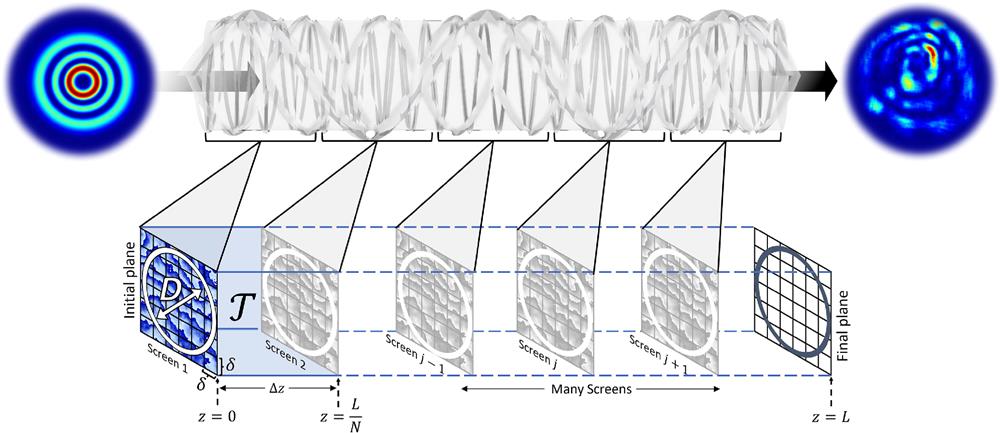
Fig. 2. The unit cell: the first turbulent screen is placed at the beginning of the channel, at z=0, with subsequent screens placed a distance Δz=L/N away from the prior, where N is the number of turbulent phase screens used. Each phase screen and distance form a unit cell, the first highlighted in blue, forming N unit cells over the complete path length of z=L. The operator for each unit cell T is identical, so we need only consider the first unit cell. The initial plane is discretized into pixels with side length δ, and turbulence is simulated with a strength characterized by the ratio D/r0, where D is the aperture of the inscribed circle and r0 is the Fried parameter. The operator describes the action of an imprinted turbulent phase on the beam, followed by vacuum propagation over a distance Δz.

Fig. 3. Eigenmodes of turbulence: the numerically calculated eigenmodes of turbulence, showing the first five modes (columns) as a function of turbulence strength (rows). The insets show the phase profile. All eigenmodes were calculated for a total propagation path of 100 m through weak, medium, and strong turbulence as defined by the Rytov variance (σR2) and Fried parameter (r0). The first two rows show eigenmodes of weak turbulence with σR2=0.5 and r0=1.8mm. The next two rows show eigenmodes of medium turbulence with σR2=1 and r0=1.2mm. The last row shows eigenmodes of strong turbulence with σR2=1.5 and r0=0.91mm.

Fig. 4. Invariance of eigenmodes under numerical propagation through turbulence. The (a) eigenmodes and (b) LG modes after numerical propagation through weak, medium, and strong turbulence through a channel equivalent to propagating over a distance of 100 m. The insets show the modes before experiencing turbulence. The numerical simulations used the split-step method with three unit cells each consisting of a turbulence screen with a given r0 followed by 33.33 m of propagation. Weak turbulence was characterized by σR2=0.5 and r0=1.8mm, medium turbulence by σR2=1 and r0=1.2mm, and strong turbulence by σR2=1.5 and r0=0.91mm.

Fig. 5. Cross-talk-free transmission: simulated cross-talk matrices for OAM (a) modes ℓ∈[0,4] and (b) eigenmodes with insets showing the intensity of the beams. The eigenmodes are unchanged and remain orthogonal, whereas the OAM modes scatter into each other. Turbulence results shown for D/r0=2 with a total path length of 100 m and a beam waist parameter for the OAM beams of w0=6.67mm.

Fig. 6. Eigenmodes of turbulence through an unperturbed, uniform medium. (a) The Laguerre–Gaussian modes propagate through free-space unaberrated, as they are solutions to the free-space paraxial Helmholtz equation. The eigenmodes of (b) weak, (c) medium, and (d) strong turbulence, while still recognizable, show noticeable changes when passing through a channel with no turbulence. The insets show the modes before propagation, and the larger images show the modes after propagation through a 100-m free-space channel with no turbulence. Weak turbulence was characterized by σR2=0.5 and r0=1.8mm, medium turbulence by σR2=1 and r0=1.2mm, and strong turbulence by σR2=1.5 and r0=0.91mm.

Fig. 7. Eigenmodes of a slant path: (a) the initial eigenmodes and (b) those after propagation through a slant path toward the ground. The invariance is clear, with the before and after intensity structures remarkably similar. We also note the strong similarity to free-space modes because the turbulence conditions were moderate.

Fig. 8. Experimental setup: lenses L1 and L2 expand and collimate a laser beam onto an SLM, in which a phase-only hologram of the initial beam is displayed, but implementing amplitude and phase control by complex amplitude modulation. The ideal, turbulence-free beam is generated at this plane and subsequently propagates through three turbulent screens, which are also displayed on SLMs, one example shown as an inset, each followed by 1 m of free-space propagation. The final aberrated field is captured on a CCD to image its intensity. Examples of the desired eigenmodes (calculated eigenmodes), the holograms to create them, and the measured eigenmodes without any turbulence or propagation (generated eigenmodes) are shown in the insets.

Fig. 9. Experimental eigenmodes. (a) The measured intensities of the eigenmodes of turbulence after propagating through the experimental setup. The results show eigenmodes of weak, medium, and strong turbulence. (b) The measured intensities of OAM modes after propagating through the same experimental setup with the same turbulence phase screens for comparison. The insets show the initial input mode. Weak turbulence was characterized by σR2=0.5 and r0=1.8mm, medium turbulence by σR2=1 and r0=1.2mm, and strong turbulence by σR2=1.5 and r0=0.91mm.