Robust structured light in atmospheric turbulence

Asher Klug; Cade Peters; Andrew Forbes

doi:10.1117/1.AP.5.1.016006

Abstract

Structured light is routinely used in free-space optical communication channels, both classical and quantum, where information is encoded in the spatial structure of the mode for increased bandwidth. Both real-world and experimentally simulated turbulence conditions have revealed that free-space structured light modes are perturbed in some manner by turbulence, resulting in both amplitude and phase distortions, and consequently, much attention has focused on whether one mode type is more robust than another, but with seemingly inconclusive and contradictory results. We present complex forms of structured light that are invariant under propagation through the atmosphere: the true eigenmodes of atmospheric turbulence. We provide a theoretical procedure for obtaining these eigenmodes and confirm their invariance both numerically and experimentally. Although we have demonstrated the approach on atmospheric turbulence, its generality allows it to be extended to other channels too, such as aberrated paths, underwater, and in optical fiber.

Keywords

eigenmodes orbital angular momentum structured light turbulence

1 Introduction

Free-space transmission of electromagnetic waves is crucial in many diverse applications, including sensing, detection and ranging, defense and communication, and extends over distances from the long (Earth monitoring) to the short (WiFi and LiFi). Lately, there has been a resurgence of interest in free-space optical links,1^,2 driven in part by the need for increased communication bandwidths,3^,4 with the potential to bridge the digital divide in a manner that is license free.5 Here the spatial modes of light have come to the fore, for so-called space division multiplexing6 and mode division multiplexing,7 where the spatial structure of light is used as an encoding degree of freedom. This in turn has fueled interest in structured light,8^,9 where light is tailored in all its degrees of freedom, including amplitude, phase, and polarization, enabled by a modern structured light toolkit.10

A commonly used form of structured light is that of beams carrying orbital angular momentum (OAM), where the phase spirals around the path of propagation azimuthally.11 These modes provide a (theoretically) infinite and easily realized alphabet for encoding information12^,13 and have been used extensively in optical communication (see Refs. 14 and 15 for good reviews). Vectorial combinations of such beams create inhomogeneous polarization structures16^–18 and also have found applications in free-space links.19^,20 Although these structured light fields hold tremendous potential for free-space optical communication, they are distorted by atmospheric turbulence as a phase perturbation in the near field and an amplitude, phase, and polarization perturbation in the far field.21 This corrects the myth that vectorial light is immune to atmospheric turbulence by virtue of its polarization components—it is not. What is invariant is its vectorness, how inhomogeneous the polarization structure is (but not how it looks), which can potentially be exploited for error-free optical communication.22 This modal scattering-induced cross talk decreases the information capacity of classical atmospheric transmission channels,23^–32 while reducing the degree of entanglement in quantum links.32^–41 Mitigating this remains an open challenge that has been intensely studied.

Arguments have been put forward for one mode family being more robust than another, with studies covering Bessel–Gaussian,42^–53 Hermite–Gaussian,54^–56 Laguerre–Gaussian (LG),57^–61 and Ince–Gaussian62 beams, with mixed and contradictory results. In the context of OAM, since the atmosphere itself can be thought of giving or taking OAM from the beam, it has been shown theoretically and experimentally that atmospheric turbulence distortions are independent of the original OAM mode,63 all susceptible to the deleterious effects of atmospheric turbulence, and indeed, it has been suggested that OAM is not the ideal modal carrier through turbulence.64 Vectorial structured light has been suggested to improve resilience because of the invariance of the polarization degree of freedom, but numerous studies in turbulence65^–72 have been inconclusive, with some reporting that the vectorial structure is stable,66^,67^,72 and others not.55^,68^–71 Careful inspection of the studies that report vectorial robustness in noisy channels reveals that the distances propagated were short and the strength of perturbation was low, mimicking a phase-only near-field effect where indeed little change is expected, and hence these are not true tests for robustness or invariance. Studies that claim enhanced resilience of vector modes over distances comparable to the Rayleigh length66^,72 have used the variance in the field’s intensity as a measure, a quantity that one would expect to be robust due to the fact that each polarization component behaves independently and so will have a low covariance. This failing of structured light in turbulence has led to numerous correction techniques, including novel encoding/decoding methods,73 modal diversity as an effective error-reduction scheme,74 traditional adaptive optics for pre- and postcorrection,75^–77 as well as vectorial adaptive tools,78 iterative routines,79 and deep learning models.80

Sign up for Advanced Photonics TOC. Get the latest issue of Advanced Photonics delivered right to you！Sign up now

Here we present a class of structured light whose entire structure in amplitude and phase remains invariant as it propagates through a turbulent free-space channel. We deploy an operator approach to find the eigenmodes of atmospheric turbulence, a significant departure from prior phenomenological approaches. Unlike other spatial modes, these exotically structured eigenmodes need no corrective procedures and are naturally devoid of deleterious effects, such as modal cross talk. Moreover, they are valid over long paths and strong aberrations, a regime that is no longer phase-only, and thus traditional adaptive solutions for correction fail. We demonstrate this invariance numerically and confirm it experimentally with a laboratory-simulated long path comprising weak, medium, and strong turbulence, implemented using multiple turbulent phase screens along the propagation path. Our approach offers a new pathway for exploiting structured light in turbulence and can be easily extended to arbitrary noisy channels.

2 Eigenmodes of Turbulence

2.1 Instantaneous Eigenmodes

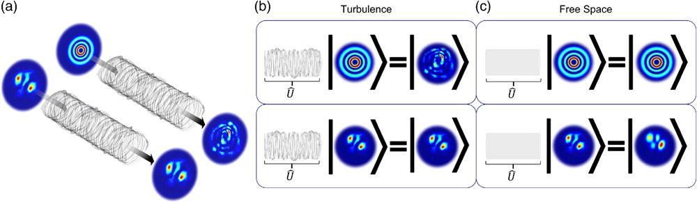
The concept we tackle here is illustrated in Fig. 1(a). Some optical field passes through an arbitrary distance of atmospheric turbulence and is treated as a continuous medium of potentially strong turbulence, which we will refer to as our channel. The conventional forms of structured light, such as LG beams are typically distorted after propagation through such a channel but are invariant to unperturbed free space. In contrast, the eigenmodes of the medium are complex forms of structured light that are invariant to the channel, emerging distortion-free but then are not eigenmodes of unperturbed free space.

Figure 1.Propagation through turbulence: (a) most common forms of structured light (such as Laguerre–Gaussian modes) become distorted when propagating through free space due to the effects of atmospheric turbulence, whereas an eigenmode of atmospheric turbulence will remain unchanged when propagating through the same channel. (b), (c) In contrast, the eigenmodes of turbulence will not be the eigenmodes of pristine free space.

In our approach to the problem, we treat the channel as an operator, $\hat{U}$ that acts on the input field to return an output field, namely, $\hat{U} u_{in} = u_{out} .$ (1)

This is illustrated in Figs. 1(b) and 1(c), with the operator and input/output fields shown schematically (note that in the absence of turbulence the operator just describes free space). The operator is unitary if the transmitting and receiving apertures are sufficiently large to accommodate the number of eigenmodes utilized, which can be approximated by its free-space limit of $N_{\max} \approx A_{t} A_{r} / (λ^{2} L^{2})$ , where $A_{t}$ and $A_{r}$ are the transmitter and receiver aperture areas separated by a distance $L$ for light of wavelength $λ$ . Equation (1) can be recast as an eigenvector problem by insisting that $u_{in} = u_{out} = | γ ⟩$ so that $\hat{U} = \sum_{i} s_{i} | γ_{i} ⟩ ⟨ γ_{i} | .$ (2)

The challenge is to find these eigenvectors $| γ_{i} ⟩$ by decomposition of the channel operator as a transmission matrix with elements $U_{i j}$ that maps the input to the output, i.e., $u_{i} = \sum_{j} U_{i j} u_{j}$ . This is a variant of singular value decomposition (SVD), which solves the eigenvector equation at two planes for two different sets of modes.81 This ensures orthogonality at the receiver by allowing the optical fields to evolve in transmission, say from modes $| ϕ_{i} ⟩$ at the transmitter to $| ψ_{i} ⟩$ at the receiver, but at the expense of invariance. We wish to find the modes that are invariant (robust) to the channel, the true eigenmodes of the channel, so that transmitter and receiver share a common mode set. Because of the unitarity of the problem, the eigenvector equation is numerically stable and can be solved by a variety of standard numerical tools, so the task is to decompose the channel operator as matrix elements. There are a variety of approaches to do this, with successful theoretical demonstrations including using SVD in turbulence with OAM and pixel modes at the transmitter and receiver,82^,83 and experimental demonstrations using point sources for eigenmodes of scattering media.84^,85 In the language of quantum mechanics, the nature of the problem lends itself to a process tomography of the channel,86 which by the isomorphism of channel and state means that a quantum state tomography87 will completely retrieve the channel matrix, as shown in quantum channels of complex optical fiber88 as well as in channels through turbulence.89^,90 We believe that this is a promising avenue to explore, as it may offer benefits over the classical approach, which typically probes the channel one mode at a time. Nevertheless, the point is that standard tools exist to tackle the problem both experimentally and computationally.

In our work, we will use the pixel basis to express the eigenmodes, inspired by the form of the paraxial free-space Green’s function. The channel tomography, however, can be done in any complete and orthogonal basis for sending and receiving modes, to reconstruct a channel matrix $A = P U Q^{†}$ , where $P$ and $Q$ are the unitary matrices that perform the basis transformations, which, following the earlier example, might be $Q = \sum_{p} | ϕ_{p} ⟩ ⟨ γ_{p} |$ and $P = \sum_{q} | ψ_{q} ⟩ ⟨ γ_{q} |$ , from which $U$ can be again deduced.

2.2 Time-Averaged Eigenmodes

The analysis in the previous section assumed that the channel matrix was fixed at some instant in time, or equivalently, that the light transit time is much shorter than the coherence time of the turbulence. It is instructive to consider what might happen if one instead considers a time-averaged result. Turbulence is a stochastic process in which the refractive index of the Earth’s atmosphere varies according to well-known statistics, having zero mean and some nonzero variance. To see the impact of averaging over many different instances of turbulence on the robustness of modes, we use the Helmholtz equation in the nonparaxial form through a thick and varying medium defined by the function $δ n (r)$ , $(\nabla^{2} + k^{2}) V = - 2 k^{2} δ n V,$ (3)which has the solution $V (r^{'}) = 2 k^{2} \int d^{3} r G (r, r^{'}) V (r) δ n (r),$ (4)with $G (r, r^{'}) = \exp (i k ‖ r - r^{'} ‖) / 4 π ‖ r - r^{'} ‖$ being the free-space Green’s function and $r = (x, z)$ . Taking the ensemble average and using the result that $⟨ δ n V ⟩ = A ⟨ V ⟩$ ,91 we find $⟨ V (r^{'}) ⟩ = 2 k^{2} A \int d^{3} r G (r, r^{'}) ⟨ V (r) ⟩,$ (5)where the constant $A$ is related to the covariance of the refractive index fluctuations. We recognize that Eq. (5) is identical to the usual, zero-turbulence Fresnel integral, up to a constant. Therefore, the averaged eigenmodes should be solutions to the free space, no turbulence, case. In other words, if the channel involves some form of averaging, say at the detector, then the best mode set in this case is identically the traditional free-space modes in various geometries, e.g., the Hermite–Gaussian and LG modes.

3 Numerical Simulation: Multiple Phase Screen Example

Conceptually, one can imagine that the real path through turbulence is subdivided into many units, each containing a single phase-only turbulent screen and a zero turbulence propagation path of length $Δ z$ . We realize that in the language of operators, the action of each unit on some field is given by the product of the operators for turbulence and free-space propagation, which we denote by $T$ . This picture serves to confirm that the complete channel operator can be treated as unitary, since it can be written as a product of unitary operators. We will now use this approach by way of example to build up a turbulence operator for the long/thick medium because (in the absence of a real-world channel) it lends itself directly to numerical testing and experimental verification of the concept in the laboratory.

To begin, we note that the effects of turbulence are mathematically captured in the stochastic refractive index $n = 1 + δ n$ , where $δ n$ is the random variation in the refractive index of the Earth’s atmosphere. It is assumed that $δ n$ has a zero mean value, i.e., $⟨ δ n ⟩ = 0$ , and that the variation is small, so $| δ n | ≪ 1$ . The introduction of this varying term produces the stochastic paraxial Helmholtz equation for a field $V (x, y, z)$ , $(\nabla_{t}^{2} + 2 i k \partial_{z} + 2 k^{2} δ n) V = 0,$ (6)where $\nabla_{t}^{2}$ is the transverse Laplacian, and $k = 2 π / λ$ is the wavenumber for wavelength $λ$ .

Equation (6) can be solved numerically according to the split-step method,92 illustrated in Fig. 2. Multiple random phase screens are placed at various distances along the beam’s propagation path. Importantly, each screen is in the weak turbulence limit and contributes a random phase $Θ_{j}$ , where $j$ labels the $j$ ’th screen, so that a single screen approximation is valid, but the sum of many such screens can lead to medium or even strong turbulence. In general, the screens at each distance are different, but for pedagogical reasons, we start with a simple example (to illustrate the concept) where we imagine that the path is subdivided into identical units, each containing such a single screen and a zero turbulence propagation path of length $Δ z$ . The action of $T$ on a field $V$ is given by the Huygen–Fresnel integral with a turbulent phase factor, $T V \equiv \int d^{2} x g (x, x^{'}; Δ z) \exp (i Θ) V (x, z = 0),$ (7)where $g (x, x^{'}; Δ z) = \frac{1}{i λ Δ z} \exp (\frac{i π}{λ Δ z} {‖ x - x^{'} ‖}^{2})$ (8)is the paraxial free-space Green’s function and $x$ , $x^{'}$ are the two-dimensional coordinates of the initial and final planes, respectively. We then discretize $x$ and $x^{'}$ into grids of $N \times N$ points. The coordinates are labeled $x \equiv (x_{α}, y_{β})$ and $x^{'} \equiv (x_{μ}, y_{ν})$ , so that $T$ is given by $T_{μ ν α β} = \frac{1}{i λ Δ z} \exp (\frac{i π}{λ Δ z} {(x_{μ} - x_{α})}^{2}) \times \exp (\frac{i π}{λ Δ z} {(y_{ν} - y_{β})}^{2}) \exp (i Θ (x_{α}, y_{β})) .$ (9)

Figure 2.The unit cell: the first turbulent screen is placed at the beginning of the channel, at $z = 0$ , with subsequent screens placed a distance $Δ z = L / N$ away from the prior, where $N$ is the number of turbulent phase screens used. Each phase screen and distance form a unit cell, the first highlighted in blue, forming $N$ unit cells over the complete path length of $z = L$ . The operator for each unit cell $T$ is identical, so we need only consider the first unit cell. The initial plane is discretized into pixels with side length $δ$ , and turbulence is simulated with a strength characterized by the ratio $D / r_{0}$ , where $D$ is the aperture of the inscribed circle and $r_{0}$ is the Fried parameter. The operator describes the action of an imprinted turbulent phase on the beam, followed by vacuum propagation over a distance $Δ z$ .

An eigenmode $E$ is then a solution to the tensor eigenvalue equation, $γ_{n} E_{μ ν}^{n} = T_{μ ν α β} E_{α β}^{n},$ (10)where $γ_{n}$ is the eigenvalue of the $n$ ’th eigenmode. Repeated indices are implicitly summed over and $E_{μ ν} \equiv E (x_{μ}, y_{ν})$ . To convert the above tensor equation into the usual matrix–vector form, we specify a mapping $ρ$ that acts on the indices $(α, β)$ and $(μ, ν)$ and “counts” them, first by columns and then by rows, such that $ρ (1, 1) = 1, \dots, ρ (N, 1) = N, ρ (1, 2) = N + 1$ up to $ρ (N, N) = N^{2}$ . This mapping lets us rewrite Eq. (10) as $γ_{n} E_{i}^{n} = T_{i j} E_{j}^{n},$ (11)since $ρ (α, β) = j$ and $ρ (μ, ν) = i$ . This equation can be routinely solved using numerical methods to find the eigenmodes of the unit cell operator. The action of the full channel is then described by the product $T_{n} \dots T_{1}$ of repeated unit cells, and as per the definition of eigenmodes, they remain invariant, regardless of the number of operators applied. To simulate more realistic conditions that change from cell to cell, the individual operators can be set appropriately so that in general $T_{n} \neq T_{n + 1}$ , but the product of operators still holds true.

3.1 Numerical Results

We follow the split-step approach shown in Fig. 2 to calculate the eigenmodes and numerically propagate them through atmospheric turbulence. For clarity and brevity, we show only the low-order eigenmodes and use the OAM modes as our point of comparison. We describe the turbulence conditions by Fried’s parameter $r_{0} = {(0.423 k^{2} C_{n}^{2} L)}^{- 3 / 5}$ and the Rytov variance $σ_{R}^{2} = 1.23 C_{n}^{2} k^{7 / 6} L^{11 / 6}$ using the plane-wave approximations93 over a path of length $L$ . These parameters are given in the captions of all results.

Examples of the intensity and phase of the eigenmodes are shown in Fig. 3 for various examples of turbulence. Here the first five eigenmode solutions are shown in Fig. 3, increasing from left to right, with the rows corresponding to the turbulence strength, increasing from top to bottom. Although these are complex forms of structured light, as eigenmodes of turbulence they should be invariant after propagation through a turbulent atmosphere. To test this, we propagate OAM carrying LG modes and the eigenmodes through various scenarios of turbulence over a 100-m path length, with the results shown in Fig. 4. OAM modes were selected, as they are very popular forms of structured light used in free-space studies. Their popularity, however, is not commensurate with their robustness in turbulence, as their phase profiles are sensitive to atmospheric distortions. We see that while the OAM modes are distorted (as expected), the eigenmodes are robust. This can be quantified by performing a modal analysis94 at the end of the turbulent channel, as would be the case in optical communication at the receiver. In Fig. 5, we see that while the cross talk is substantial for OAM modes when propagated through turbulence, evident from the many off-diagonal terms, the eigenmode cross-talk matrix remains diagonal after the same channel, for minimal cross talk. It is useful to study the behavior of the eigenmodes of turbulence as they propagate through a channel with no turbulence and that is absent of any other perturbations. LG and Hermite–Gaussian modes are eigenmodes of such a channel and thus will propagate through it unperturbed. This can be seen in Fig. 6(a) where several LG modes of increasing OAM numerically propagate through a 100 m free-space channel and show no aberrations. The eigenmodes of weak, medium, and strong turbulence [in Figs. 6(b)–6(d), respectively] are also propagated through this channel. They show very noticeable changes in their intensity distributions, thus demonstrating that they are not eigenmodes of free space. However, the change they undergo in free space is not so significant as to make them unrecognizable, and they retain many of their original features, such as a general pattern and the number of lobes. When comparing this to Fig. 4, it appears that the changes undergone by eigenmodes of turbulence in free space are less severe than changes undergone by the eigenmodes of free space in turbulence.

Figure 3.Eigenmodes of turbulence: the numerically calculated eigenmodes of turbulence, showing the first five modes (columns) as a function of turbulence strength (rows). The insets show the phase profile. All eigenmodes were calculated for a total propagation path of 100 m through weak, medium, and strong turbulence as defined by the Rytov variance ( $σ_{R}^{2}$ ) and Fried parameter ( $r_{0}$ ). The first two rows show eigenmodes of weak turbulence with $σ_{R}^{2} = 0.5$ and $r_{0} = 1.8 mm$ . The next two rows show eigenmodes of medium turbulence with $σ_{R}^{2} = 1$ and $r_{0} = 1.2 mm$ . The last row shows eigenmodes of strong turbulence with $σ_{R}^{2} = 1.5$ and $r_{0} = 0.91 mm$ .

Figure 4.Invariance of eigenmodes under numerical propagation through turbulence. The (a) eigenmodes and (b) LG modes after numerical propagation through weak, medium, and strong turbulence through a channel equivalent to propagating over a distance of 100 m. The insets show the modes before experiencing turbulence. The numerical simulations used the split-step method with three unit cells each consisting of a turbulence screen with a given $r_{0}$ followed by 33.33 m of propagation. Weak turbulence was characterized by $σ_{R}^{2} = 0.5$ and $r_{0} = 1.8 mm$ , medium turbulence by $σ_{R}^{2} = 1$ and $r_{0} = 1.2 mm$ , and strong turbulence by $σ_{R}^{2} = 1.5$ and $r_{0} = 0.91 mm$ .

Figure 5.Cross-talk-free transmission: simulated cross-talk matrices for OAM (a) modes $ℓ \in [0,4]$ and (b) eigenmodes with insets showing the intensity of the beams. The eigenmodes are unchanged and remain orthogonal, whereas the OAM modes scatter into each other. Turbulence results shown for $D / r_{0} = 2$ with a total path length of 100 m and a beam waist parameter for the OAM beams of $w_{0} = 6.67 mm$ .

Figure 6.Eigenmodes of turbulence through an unperturbed, uniform medium. (a) The Laguerre–Gaussian modes propagate through free-space unaberrated, as they are solutions to the free-space paraxial Helmholtz equation. The eigenmodes of (b) weak, (c) medium, and (d) strong turbulence, while still recognizable, show noticeable changes when passing through a channel with no turbulence. The insets show the modes before propagation, and the larger images show the modes after propagation through a 100-m free-space channel with no turbulence. Weak turbulence was characterized by $σ_{R}^{2} = 0.5$ and $r_{0} = 1.8 mm$ , medium turbulence by $σ_{R}^{2} = 1$ and $r_{0} = 1.2 mm$ , and strong turbulence by $σ_{R}^{2} = 1.5$ and $r_{0} = 0.91 mm$ .

Real-world turbulent channels have differing unit cells and to illustrate such an example, we simulate a slant path from high altitude to the Earth’s surface. In this case, the turbulence strength changes as a function of altitude, and likewise, the phase screen in each cell changes.

The starting altitude of the channel was 500 m and the zenith angle was 170 deg (the zenith angle is $> 90 \deg$ , as we are propagating downward from a point of high altitude to the surface of the Earth). This corresponds to a path length of 508 m and an angle of 80 deg below the horizontal. To calculate the turbulence strength at each altitude, the Tartarski model95 was used to calculate the values for the refractive index structure constant, $C_{n}^{2} (h) = C_{n 0}^{2} h^{- b},$ (12)where $C_{n 0}^{2} = 4.16 \times 10^{- 13} m^{2 / 3}$ and $b = 4 / 3$ are constants selected to most closely fit experimental data and $h$ is the altitude. The slant path length through the atmospheric layer is given by $Δ l_{i}^{2} = Δ h_{i}^{2} + Δ z_{i}^{2}$ , where $Δ h_{i}^{2}$ is the height of the atmospheric layer and $Δ z_{i}^{2}$ is the horizontal component of the beam’s path through the layer; the channel was broken up into 14 unit cells. The phase screens were then distributed evenly along the path, and the values for $C_{n_{i}}^{2}$ were calculated for each phase screen at the position of each phase screen. The calculated eigenmodes for this example are shown in Fig. 7, where we see some striking similarity to low-order superpositions of the free-space modes. More importantly, we note that the before and after intensity structures are in good agreement, indicative of an eigenmode.

Figure 7.Eigenmodes of a slant path: (a) the initial eigenmodes and (b) those after propagation through a slant path toward the ground. The invariance is clear, with the before and after intensity structures remarkably similar. We also note the strong similarity to free-space modes because the turbulence conditions were moderate.

4 Experimental Results

The experiment, shown in Fig. 8, is conceptually divided into three parts. In the generation stage, a He–Ne laser beam (wavelength $λ = 633 nm$ ) was expanded using a $10 \times$ objective lens $L_{1}$ and then collimated by $L_{2}$ ( $f_{2} = 150 mm$ ) before being directed onto a reflective PLUTO-VIS HoloEye spatial light modulator (SLM). The initial field was generated using the Arrizón type 3 technique96 to shape the incident beam into the desired mode by complex amplitude modulation (amplitude and phase control). This field then entered the turbulent section of the setup, where it passed through three unit cells, each comprising the same random phase screen and a propagation distance of 1 m. The same phase screen was repeated for ease of calculation. In a real-world channel, the phase screens would not be correlated; however, the method would still remain unchanged, as demonstrated in the previous section. The phase screens were generated using the subharmonic random matrix transform method92 and displayed on the (phase-only) SLMs. The intensity of the perturbed field was then detected and measured on a camera (CCD). The experimental setup in Fig. 8 shows four examples of the desired (calculated) eigenmodes, the holograms to create them by complex amplitude modulation, and the experimental validation that, without any turbulence or propagation, they are created (generated eigenmodes) with high fidelity.

Figure 8.Experimental setup: lenses $L_{1}$ and $L_{2}$ expand and collimate a laser beam onto an SLM, in which a phase-only hologram of the initial beam is displayed, but implementing amplitude and phase control by complex amplitude modulation. The ideal, turbulence-free beam is generated at this plane and subsequently propagates through three turbulent screens, which are also displayed on SLMs, one example shown as an inset, each followed by 1 m of free-space propagation. The final aberrated field is captured on a CCD to image its intensity. Examples of the desired eigenmodes (calculated eigenmodes), the holograms to create them, and the measured eigenmodes without any turbulence or propagation (generated eigenmodes) are shown in the insets.

Our setup differs from conventional laboratory simulations of turbulence in that we are able to mimic a thick path, from weak to strong turbulence, whereas often only a single-phase screen is used, allowing only weak turbulence to be tested. Using our setup, we studied an effective real-world channel of $L = 100 m$ , at our wavelength of $λ = 633 nm$ and with Rytov variances of $σ_{R}^{2} = 1.5$ , 1, and 0.5, corresponding to strong, medium, and weak turbulence, with Fried parameters ( $r_{0}$ ) of 0.47, 0.62, and 0.93 mm, respectively. We required three screens for each turbulence strength, separated by a distance of 33.3 m, each with effective Fried parameters $r_{0, s} = 0.9$ , 1.2, and 1.8 mm, while maintaining a Rytov variance in each slab (segment of the channel) to be smaller than 0.9, 0.6, and 0.3, respectively. This channel was simulated on the setup shown in Fig. 8 using the Fresnel scaling procedure,97 allowing a long path to be generated within laboratory distances. The scaling factors were chosen to be: $α_{x} = α_{x^{'}} = \sqrt{0.03} \approx 0.173$ and $α_{z} = 0.03$ . This corresponded to a total path length of $L^{'} = 3 m$ and segment Fried parameters of $r_{0, s} = 0.081$ , 0.11, and 0.16 mm (see Appendix for details).

The results of OAM and the eigenmodes for weak, medium, and strong turbulence are shown in Fig. 9. The collage shows the final measured eigenmodes after the channel, with the insets showing the initial mode as prepared prior to the channel. The robustness of the eigenmodes is clearly evident, in contrast to the highly distorted OAM modes.

Figure 9.Experimental eigenmodes. (a) The measured intensities of the eigenmodes of turbulence after propagating through the experimental setup. The results show eigenmodes of weak, medium, and strong turbulence. (b) The measured intensities of OAM modes after propagating through the same experimental setup with the same turbulence phase screens for comparison. The insets show the initial input mode. Weak turbulence was characterized by $σ_{R}^{2} = 0.5$ and $r_{0} = 1.8 mm$ , medium turbulence by $σ_{R}^{2} = 1$ and $r_{0} = 1.2 mm$ , and strong turbulence by $σ_{R}^{2} = 1.5$ and $r_{0} = 0.91 mm$ .

5 Discussion

We have outlined how to find the eigenmodes of a turbulent path and demonstrated it with a laboratory-based split-step example both numerically and experimentally. These modes are eigenmodes in their truest sense, i.e., they are fixed under the action of the channel. Importantly, our approach works even when the medium is long and the aberration strong, a regime where traditional adaptive optics often fails (beyond a Rytov variance of order 1).98^,99

A natural feature of the eigenmodes is that they are channel-specific. To be useful in a real-world setting, the transmission should be faster than the coherence time of the turbulence. For typical turbulence conditions, this is always true, with the atmosphere changing on millisecond time scales (typically 1 to 10 ms), whereas the transport of light across kilometer-length scales is on the order of nanoseconds. The turbulence thus appears frozen, and numerical simulations on singular value modes have shown that they outperform adaptive solutions, even in dynamic turbulence.100 The time frames of acquiring the information to deduce the eigenmodes can be very fast. A tomography of the channel can be done by modal decomposition in any basis94 with projective holograms, which with digital micromirror devices (DMDs) and photodiodes can certainly be done on millisecond time scales. This can be improved down to microseconds (limited by the response of fast photodiodes) if the projective holograms are hard-coded, such as on a diffractive optical element or metasurface, possibly because the channel does not have to be probed in the basis of eigenmodes. Further, one can surmise that machine learning would be ideally suited to the task of anticipating the new eigenmodes in a dynamical system given the prior set, certainly appealing if the conditions are slowly changing. We take some confidence from the fact that such channel analysis is needed in multiple input multiple output (MIMO) as well as in SVD approaches, both of which have been applied to nonturbulence studies already with success. Nevertheless, it is a challenge that should not be downplayed and is certainly deserving of a full experimental study. We point out that turbulence was used here only as an extreme example, whereas the formulation of the idea is such that it will work for any long path in complex media, for instance, turbid, underwater, optical fiber, or thermally aberrated paths, all of which may change more slowly or not at all. Our analysis only considered scalar modes, whereas it is clear that vectorial superpositions would also be eigenmodes of this channel. In this way, the invariance of the inhomogeneity of vectorial light in complex channels21 could be generalized to the invariance of all properties of the field, an appealing notion for energy transport and imaging through complex systems.

6 Conclusion

The search for robust states of structured light in noisy channels is a pressing challenge, promising enhanced channel capacity and reach. Here using free-space and atmospheric turbulence as our example, we have outlined a theoretical approach to finding the complex forms of structured light which are invariant under propagation through the atmosphere, the true eigenmodes of turbulence, and confirmed its validity both numerically and experimentally. These exotically structured eigenmodes need no corrective procedures, are naturally devoid of deleterious effects, and are valid over any path length in the medium. Our approach offers a new pathway for exploiting structured light in turbulence and can be easily extended to other noisy channels, such as underwater and optical fiber.

7 Appendix

Some channel parameters, such as path length, are highly restricted in the laboratory setting. This presents an apparent difficulty in experimentally verifying the eigenmodes. However, a scaling procedure exists97 that allows us to verify real-world channels in the laboratory. This procedure is presented below.

The Fresnel integral for the full (real-world) channel of length $L$ is $U_{f} (r, L) = \frac{\exp (i k L)}{i λ L} \int d^{2} r^{'} U_{i} (r^{'}) \exp (\frac{i π}{λ L} {‖ r - r^{'} ‖}^{2}) .$ (13)

We then apply the following scaling parameters: $r_{lab} = α_{x} r, r_{lab}^{'} = α_{r^{'}} r^{'}$ , and $L^{'} = α_{z} L$ , where $r_{lab}$ and $r_{lab}^{'}$ are the coordinates used in the experiment. The diffraction integral becomes $U_{f} (\frac{r_{lab}}{α_{r}}) = \frac{\exp (i k L^{'} / α_{z})}{i α_{r^{'}} λ L^{'}} \int d^{2} {r^{'}}_{lab} U_{i} (\frac{{r^{'}}_{lab}}{α_{r^{'}}}) \times \exp (\frac{i π α_{z}}{λ L^{'}} {‖ \frac{r_{lab}}{α_{r}} - \frac{{r^{'}}_{lab}}{α_{r^{'}}} ‖}^{2}) .$ (14)

To keep the diffraction equivalent with these scaled coordinates, we require the Fresnel number, $F = \frac{π D_{i} D_{f}}{4 λ L}$ (15)to be the same in both the full and scaled-down cases, where $D_{i}$ and $D_{f}$ are the aperture diameters in the initial and final planes, respectively. This sets $α_{r} α_{r^{'}} = α_{z}$ , and the diffraction integral becomes $\frac{\exp (i k L^{'} (1 - \frac{1}{α_{z}}))}{α_{r}} U_{f} (\frac{r_{lab}}{α_{r}}) = \exp (- \frac{i π r_{lab}^{2}}{λ f_{r}}) \frac{\exp (i k L^{'})}{i λ L^{'}} \times \int d^{2} r_{lab}^{'} U_{i} (\frac{r_{lab}^{'}}{α_{r^{'}}}) \exp (- \frac{π (r_{lab}^{'})^{2}}{λ f_{r^{'}}}) \exp (\frac{i π}{λ L^{'}} ‖ r_{lab} - r_{lab}^{'} ‖),$ (16)where $f_{r} = \frac{L^{'}}{1 - α_{r^{'}} / α_{r}},$ (17) $f_{r^{'}} = \frac{L^{'}}{1 - α_{r} / α_{r^{'}}} .$ (18)

Setting $α_{r} = α_{r^{'}}$ means that the final and initial planes have the same size in the laboratory setting and $f_{r, r^{'}} \to \infty$ . Ignoring constant phase factors that arise due to scaling, the final Fresnel integral becomes $U_{f} (\frac{r_{lab}}{α_{r}}) = \frac{α_{r} \exp (i k L^{'})}{i λ L^{'}} \int d^{2} r_{lab} U_{i} (\frac{r_{lab}^{'}}{α_{r^{'}}}) \times \exp (\frac{i π}{λ L^{'}} ‖ r_{lab} - r_{lab}^{'} ‖) .$ (19)

Andrew Forbes is a professor within the School of Physics at University of the Witwatersrand, South Africa, where in 2015 he established the Structured Light Laboratory. He is active in promoting photonics in Africa, as a founding member of the Photonics Initiative of South Africa and initiator of South Africa’s Quantum Roadmap. He is a fellow of SPIE, Optica, and the South African Institute of Physics (SAIP), and an elected member of the Academy of Science of South Africa. His outstanding contributions to the field have been recognized by many awards, including the Sang Soo Lee Award from Optica and the Optical Society of Korea, the Georg Forster Research Award from the Alexander von Humboldt Foundation, and the SAIP Gold Medal, the highest award for physics in South Africa.

Biographies of the other authors are not available.

References

[1] A. Trichili et al. Communicating using spatial mode multiplexing: potentials, challenges, and perspectives. IEEE Commun. Surv. Tutorials, 21, 3175-3203(2019).

[2] A. Trichili et al. Roadmap to free space optics. J. Opt. Soc. Am. B, 37, A184-A201(2020).

[3] D. J. Richardson. Filling the light pipe. Science, 330, 327-328(2010).

[4] D. Richardson, J. Fini, L. Nelson. Space-division multiplexing in optical fibres. Nat. Photonics, 7, 354-362(2013).

[5] M. P. Lavery et al. Tackling Africa’s digital divide. Nat. Photonics, 12, 249-252(2018).

[6] G. Li et al. Space-division multiplexing: the next frontier in optical communication. Adv. Opt. Photonics, 6, 413-487(2014).

[7] S. Berdagué, P. Facq. Mode division multiplexing in optical fibers. Appl. Opt., 21, 1950-1955(1982).

[8] A. Forbes, M. de Oliveira, M. R. Dennis. Structured light. Nat. Photonics, 15, 253-262(2021).

[9] A. Forbes. Structured light: tailored for purpose. Opt. Photonics News, 31, 24-31(2020).

[10] Y. Shen. Rays, waves, SU(2) symmetry and geometry: toolkits for structured light. J. Opt., 23, 124004(2021).

[11] M. J. Padgett. Orbital angular momentum 25 years on. Opt. Express, 25, 11265-11274(2017).

[12] G. Gibson, M. J. Courtial, J. Padgett. Free-space information transfer using light beams carrying orbital angular momentum. Opt. Express, 12, 5448-5456(2004).

[13] J. Wang et al. Terabit free-space data transmission employing orbital angular momentum multiplexing. Nat. Photonics, 6, 488-496(2012).

[14] A. E. Willner et al. Optical communications using orbital angular momentum beams. Adv. Opt. Photonics, 7, 66-106(2015).

[15] A. E. Willner et al. Orbital angular momentum of light for communications. Appl. Phys. Rev., 8, 041312(2021).

[16] Q. Zhan. Cylindrical vector beams: from mathematical concepts to applications. Adv. Opt. Photonics, 5, 1-57(2009).

[17] C. Rosales-Guzmán, B. Ndagano, A. Forbes. A review of complex vector light fields and their applications. J. Opt., 20, 123001(2018).

[18] E. Otte, C. Alpmann, C. Denz. Polarization singularity explosions in tailored light fields. Laser Photonics Rev., 12, 1700200(2018).

[19] G. Milione et al. Gbit/s mode division multiplexing over free space using vector modes and a q-plate mode (de)multiplexer. Opt. Lett., 40, 1980-1983(2015).

[20] A. Sit et al. High-dimensional intracity quantum cryptography with structured photons. Optica, 4, 1006-1010(2017).

[21] I. Nape et al. Revealing the invariance of vectorial structured light in complex media. Nat. Photonics, 16, 538-546(2022).

[22] K. Singh et al. A robust basis for multi-bit optical communication with vectorial light(2022).

[23] J. A. Anguita, M. A. Neifeld, B. V. Vasic. Turbulence-induced channel crosstalk in an orbital angular momentum-multiplexed free-space optical link. Appl. Opt., 47, 2414-2429(2008).

[24] Y. Ren et al. Experimental characterization of a 400 Gbit/s orbital angular momentum multiplexed free-space optical link over 120 m. Opt. Lett., 41, 622-625(2016).

[25] M. Krenn et al. Communication with spatially modulated light through turbulent air across Vienna. New J. Phys., 16, 113028(2014).

[26] Y. Zhao et al. Experimental demonstration of 260-meter security free-space optical data transmission using 16-QAM carrying orbital angular momentum (OAM) beams multiplexing, Th1H–3.(2016).

[27] B. Rodenburg et al. Influence of atmospheric turbulence on states of light carrying orbital angular momentum. Opt. Lett., 37, 3735-3737(2012).

[28] M. Krenn et al. Twisted light transmission over 143 km. Proc. Natl. Acad. Sci. U. S. A., 113, 13648-13653(2016).

[29] L. Zhang et al. Mode-dependent crosstalk and detection probability of orbital angular momentum of optical vortex beam through atmospheric turbulence. J. Opt., 22, 075607(2020).

[30] M. Malik et al. Influence of atmospheric turbulence on optical communications using orbital angular momentum for encoding. Opt. Express, 20, 13195-13200(2012).

[31] C. Chen et al. Changes in orbital-angular-momentum modes of a propagated vortex gaussian beam through weak-to-strong atmospheric turbulence. Opt. Express, 24, 6959-6975(2016).

[32] G. A. Tyler, R. W. Boyd. Influence of atmospheric turbulence on the propagation of quantum states of light carrying orbital angular momentum. Opt. Lett., 34, 142-144(2009).

[33] C. Paterson. Atmospheric turbulence and orbital angular momentum of single photons for optical communication. Phys. Rev. Lett., 94, 153901(2005).

[34] A. K. Jha, G. A. Tyler, R. W. Boyd. Effects of atmospheric turbulence on the entanglement of spatial two-qubit states. Phys. Rev. A, 81, 053832(2010).

[35] A. Hamadou Ibrahim et al. Orbital-angular-momentum entanglement in turbulence. Phys. Rev. A, 88, 012312(2013).

[36] C. Gopaul, R. Andrews. The effect of atmospheric turbulence on entangled orbital angular momentum states. New J. Phys., 9, 94(2007).

[37] Y. Zhang et al. Experimentally observed decay of high-dimensional entanglement through turbulence. Phys. Rev. A, 94, 032310(2016).

[38] B.-J. Pors et al. Transport of orbital-angular-momentum entanglement through a turbulent atmosphere. Opt. Express, 19, 6671-6683(2011).

[39] S. K. Goyal et al. The effect of turbulence on entanglement-based free-space quantum key distribution with photonic orbital angular momentum. J. Opt., 18, 064002(2016).

[40] N. D. Leonhard, V. N. Shatokhin, A. Buchleitner. Universal entanglement decay of photonic-orbital-angular-momentum qubit states in atmospheric turbulence. Phys. Rev. A, 91, 012345(2015).

[41] G. Sorelli et al. Entanglement protection of high-dimensional states by adaptive optics. New J. Phys., 21, 023003(2019).

[42] N. Mphuthi, R. Botha, A. Forbes. Are bessel beams resilient to aberrations and turbulence?. J. Opt. Soc. Am. A, 35, 1021-1027(2018).

[43] N. Mphuthi et al. Free-space optical communication link with shape-invariant orbital angular momentum Bessel beams. Appl. Opt., 58, 4258-4264(2019).

[44] I. P. Lukin. Mean intensity of vortex Bessel beams propagating in turbulent atmosphere. Appl. Opt., 53, 3287-3293(2014).

[45] B.-S. Chen, J.-X. Pu. Propagation of Gauss–Bessel beams in turbulent atmosphere. Chin. Phys. B, 18, 1033(2009).

[46] K. Zhu et al. Propagation of Bessel–Gaussian beams with optical vortices in turbulent atmosphere. Opt. Express, 16, 21315-21320(2008).

[47] W. Nelson et al. Propagation of Bessel and Airy beams through atmospheric turbulence. J. Opt. Soc. Am. A, 31, 603-609(2014).

[48] N. Ahmed et al. Mode-division-multiplexing of multiple Bessel–Gaussian beams carrying orbital-angular-momentum for obstruction-tolerant free-space optical and millimetre-wave communication links. Sci. Rep., 6, 22082(2016).

[49] M. Cheng et al. Channel capacity of the OAM-based free-space optical communication links with Bessel–Gauss beams in turbulent ocean. IEEE Photonics J., 8, 7901411(2016).

[50] T. Doster, A. T. Watnik. Laguerre–Gauss and Bessel–Gauss beams propagation through turbulence: analysis of channel efficiency. Appl. Opt., 55, 10239-10246(2016).

[51] R. J. Watkins et al. Experimental probing of turbulence using a continuous spectrum of asymmetric OAM beams. Opt. Express, 28, 924-935(2020).

[52] C. Vetter et al. Realization of free-space long-distance self-healing Bessel beams. Laser Photonics Rev., 13, 1900103(2019).

[53] Y. Yuan et al. Beam wander relieved orbital angular momentum communication in turbulent atmosphere using Bessel beams. Sci. Rep., 7, 42276(2017).

[54] M. A. Cox et al. The resilience of Hermite– and Laguerre–Gaussian modes in turbulence. J. Lightwave Technol., 37, 3911-3917(2019).

[55] B. Ndagano et al. Comparing mode-crosstalk and mode-dependent loss of laterally displaced orbital angular momentum and Hermite–Gaussian modes for free-space optical communication. Opt. Lett., 42, 4175-4178(2017).

[56] S. Restuccia et al. Comparing the information capacity of Laguerre–Gaussian and Hermite–Gaussian modal sets in a finite-aperture system. Opt. Express, 24, 27127-27136(2016).

[57] A. Trichili et al. Optical communication beyond orbital angular momentum. Sci. Rep., 6, 27674(2016).

[58] N. Zhao et al. Capacity limits of spatially multiplexed free-space communication. Nat. Photonics, 9, 822-826(2015).

[59] Y. Zhou et al. Using all transverse degrees of freedom in quantum communications based on a generic mode sorter. Opt. Express, 27, 10383-10394(2019).

[60] G. Xie et al. Experimental demonstration of a 200-Gbit/s free-space optical link by multiplexing Laguerre–Gaussian beams with different radial indices. Opt. Lett., 41, 3447-3450(2016).

[61] L. Li et al. Power loss mitigation of orbital-angular-momentum-multiplexed free-space optical links using nonzero radial index Laguerre–Gaussian beams. J. Opt. Soc. Am. B, 34, 1-6(2017).

[62] X. Gu, L. Chen, M. Krenn. Phenomenology of complex structured light in turbulent air. Opt. Express, 28, 11033-11050(2020).

[63] A. Klug, I. Nape, A. Forbes. The orbital angular momentum of a turbulent atmosphere and its impact on propagating structured light fields. New J. Phys., 23, 093012(2021).

[64] D. A. Miller. Better choices than optical angular momentum multiplexing for communications. Proc. Natl. Acad. Sci. U. S. A., 114, E9755-E9756(2017).

[65] M. A. Cox et al. Structured light in turbulence. IEEE J. Sel. Top. Quantum Electron., 27, 7500521(2020).