
Li Xiang, Wang Lixin, Duan Zhiqiang. Application of Improved Adaptive Wavelet Noise Reduction in Laser Gyroscope Signal Processing[J]. Laser & Optoelectronics Progress, 2020, 57(21): 210401
- Laser & Optoelectronics Progress
- Vol. 57, Issue 21, 210401 (2020)
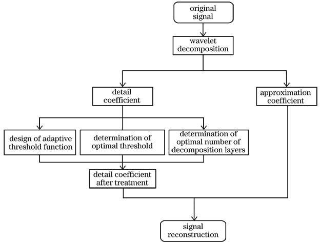
Fig. 1. Flow chart of wavelet noise reduction
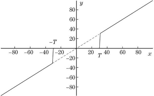
Fig. 2. Hard threshold function
Fig. 3. Soft threshold function
Fig. 4. Adaptive threshold function
Fig. 5. Curves comparison of different functions
Fig. 6. Process of determining optimal number of decomposition levels
Fig. 7. Signal data collected by three-axis laser gyroscope. (a) X-axis; (b) Y-axis; (c) Z-axis
Fig. 8. Allan variance logarithm curves of static raw data
Fig. 9. Comparison of effects of commonly used noise reduction methods. (a) Original signal; (b) TAWF; (c) standard KF; (d) IAWF
Fig. 10. Allan variance curves of noise reduction signal under different methods
Fig. 11. Effect of IAWF method after processing noise
Fig. 12. Test device for experimental car
Fig. 13. Noise reduction effect of different filtering methods
Fig. 14. Calculation results of entropy values. (a) Energy entropy of detail coefficient; (b) energy entropy of approximate coefficient; (c) energy entropy of detail ratio
Fig. 15. Dynamic noise reduction effect under different decomposition layers
Fig. 16. Detailed enlarged view of Fig. 15
|
Table 1. Noise figures of original signal
|
Table 2. Noise figures of signal

Set citation alerts for the article
Please enter your email address
© Copyright 2018-2021 | Chinese Laser Press. All Rights Reserved 沪ICP备15018463号-20