【AIGC One Sentence Reading】:This study introduces a method using optical frequency combs to characterize and linearize laser chirp dynamics, enhancing coherent ranging and spectroscopy performance without additional linearization units.
【AIGC Short Abstract】:In this study, we introduce a method utilizing an optical frequency comb to characterize and linearize laser chirp dynamics. This approach allows for precise tracking of instantaneous laser frequency over a wide bandwidth. We demonstrate its application in coherent ranging, eliminating the need for additional linearization units. This novel technique enhances laser spectroscopy and sensing capabilities, crucial for advancing high-performance applications.
Note: This section is automatically generated by AI . The website and platform operators shall not be liable for any commercial or legal consequences arising from your use of AI generated content on this website. Please be aware of this.
Abstract
Tunable lasers, with the ability to continuously vary their emission wavelengths, have found widespread applications across various fields such as biomedical imaging, coherent ranging, optical communications, and spectroscopy. In these applications, a wide chirp range is advantageous for large spectral coverage and high frequency resolution. Besides, the frequency accuracy and precision also depend critically on the chirp linearity of the laser. While extensive efforts have been made on the development of many kinds of frequency-agile, widely tunable, narrow-linewidth lasers, wideband yet precise methods to characterize and linearize laser chirp dynamics are also demanded. Here we present an approach to characterize laser chirp dynamics using an optical frequency comb. The instantaneous laser frequency is tracked over terahertz bandwidth at 1 MHz intervals. Using this approach we calibrate the chirp performance of 12 tunable lasers from Toptica, Santec, New Focus, EXFO, and NKT that are commonly used in fiber optics and integrated photonics. In addition, with acquired knowledge of laser chirp dynamics, we demonstrate a simple frequency-linearization scheme that enables coherent ranging without any optical or electronic linearization unit. Our approach not only presents novel wideband, high-resolution laser spectroscopy, but is also critical for sensing applications with ever-increasing requirements on performance.
1. INTRODUCTION
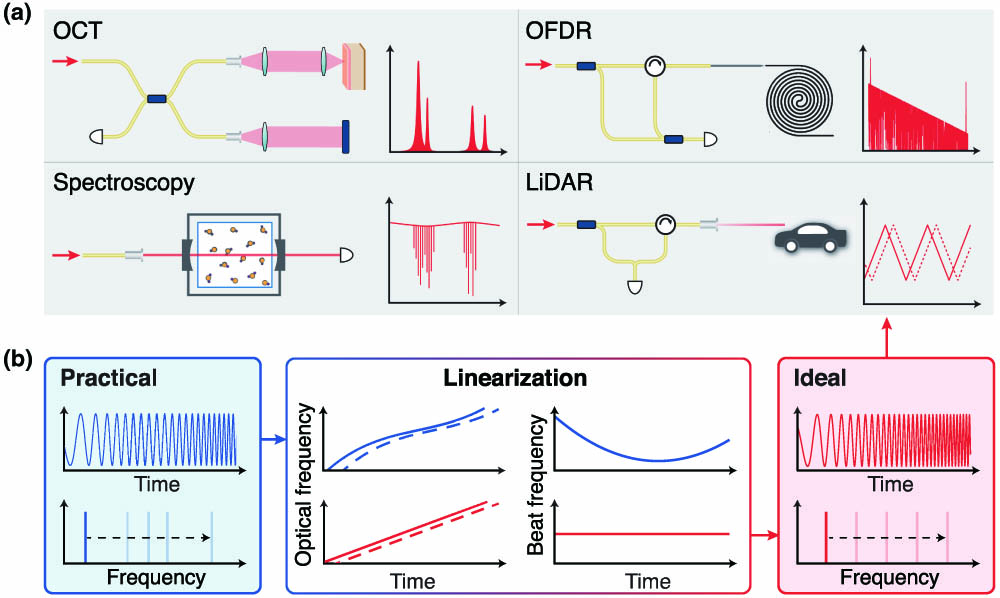
Tunable lasers, which have the ability to dynamically adjust their emission wavelength, have found widespread applications in a variety of industrial and scientific fields. For example, as shown in Fig. 1(a), in biomedical imaging, optical coherence tomography (OCT) [1–3] employs a widely tunable laser that provides a noninvasive and noncontact imaging modality for high-resolution, two-dimensional cross-sectional and three-dimensional volumetric imaging of tissue structures. In optical communication systems, optical frequency-domain reflectometry (OFDR) [4,5] uses tunable lasers for broadband loss and dispersion characterization. In laser spectroscopy, tunable diode laser absorption spectroscopy (TDLAS) [6–8] allows compound analysis of gases, as well as their conditions such as concentration, pressure, temperature, and velocity. For light detection and ranging (LiDAR), frequency-modulated continuous-wave (FMCW) LiDAR [9–14] uses a tunable laser to measure the distance (based on the time of flight) and speed (based on the Doppler effect) of a moving object.
Figure 1.Applications and principle of widely tunable lasers. (a) Applications requiring linearly chirping lasers. OCT, optical coherence tomography; OFDR, optical frequency-domain reflectometry; LiDAR, light detection and ranging. (b) Principle of laser chirp linearization. An ideal laser chirps at a constant rate. However, in reality, the actual chirp rate varies. By beating the laser with its delayed part, the chirp nonlinearity in the optical domain is revealed in the radio frequency (RF) domain.
In all of these applications, as well as others, the laser chirp range determines the measurement resolution and spectral bandwidth. However, due to the nonlinearity of laser gain and dynamics, tunable lasers typically exhibit chirping nonlinearity that is particularly deteriorated for a wide chirp range, as illustrated in Fig. 1(b). As a result, the laser chirp rate deviates from the set value, which compromises the frequency resolution, precision, and accuracy in applications. Therefore, widely tunable lasers require careful characterization and linearization for demanding applications.
To track the laser chirp rate, a fiber unbalanced Mach–Zehnder interferometer (UMZI) is commonly used to calibrate the instantaneous laser frequency, e.g., in data processing [15–17], active linearization [9], and laser drive signal optimization [18]. However, for a wide chirp range, the fiber dispersion seriously reduces the calibration precision of fiber UMZIs and causes phase-instability issues, leading to insufficient accuracy for linearization. In comparison, fully stabilized optical frequency combs (OFCs) with equidistant grids of frequency lines can essentially resolve these issues [10,19–22].
Sign up for Photonics Research TOC. Get the latest issue of Photonics Research delivered right to you!Sign up now
Here we demonstrate an approach to characterize the chirp dynamics of widely tunable lasers. We apply this method on 12 lasers from Toptica, Santec, New Focus, EXFO, and NKT that are commonly used in fiber optics and integrated photonics. Using an OFC and digital band-pass filters, the instantaneous laser frequency is tracked with 1 MHz intervals over terahertz bandwidth. This allows the linearization of laser frequency with pre-calibrated chirp rate, particularly useful for coherent LiDAR.
2. PRINCIPLE AND SETUP
To measure the laser chirp rate, we use a commercial, fully stabilized, fiber-based OFC (Quantum CTek) as a frequency “ruler” [23–25] to trace the instantaneous laser frequency during chirping. In our case, the comb repetition rate and its carrier envelope offset frequency are actively locked to a rubidium atomic clock; thus the OFC is fully stabilized. Consequently, in the frequency domain, the th comb line’s frequency is unambiguously determined as .
When the laser chirps, it beats against tens of thousands of comb lines with precisely known frequency values, as shown in Fig. 2(a). Beat signals of frequencies are generated, where is the instantaneous frequency of the tunable laser at time . As the frequency comb is fully stabilized, for a mode-hop-free tunable laser, the dynamics and linearity of are projected onto the beat signals. The simplest beat signals to analyze are the two generated by the tunable laser with its two neighboring comb lines, i.e., . Experimentally, the two beat signals are recorded by an oscilloscope after passing through a low-pass filter (LPF, Mini-Circuits, ), whose 3-dB cutoff frequency is 155 MHz in our case. We denote the frequencies of the two beat signals as and ( and ). As shown in Fig. 2(b), for a continuous linear chirp, when the laser frequency passes through the comb lines sequentially, and vary in a sawtooth waveform. The time-domain waveform near is shown in the leftmost panel of Fig. 2(d), corresponding to the situation when the laser chirps across a comb line.
Figure 2.Schematic and experimental setup of laser chirp characterization. (a) Experimental setup. BPF, band-pass filter; PC, polarization controller; BPD, balanced photodetector; LPF, low-pass filter; OSC, oscilloscope. (b) Illustration of the laser frequency beating with the OFC during laser chirping at a rate of . The time traces of the two beat frequencies and () are shown. (c) Upper panel shows the instantaneous frequency of the tunable laser in the ideal (red) and actual (blue) cases. Lower panel shows the corresponding instantaneous chirp rate . (d) Flowcharts of the algorithm based on finite impulse response (FIR) band-pass filters (BPFs), to extract the instantaneous laser frequency as well as the chirp rate. The dashed lines mark the time where the laser frequency scans across a comb line. (e) The FIR filter’s center frequency is digitally set, and the instantaneous laser frequency is calculated over 1 MHz intervals.
Here, we concentrate on the analysis of , since . The dynamics and linearity of as a function of time are identical to those of the laser frequency . We process the signal and extract the instantaneous frequency value as illustrated in Fig. 2(d). A finite impulse response (FIR) band-pass filter with a specific pass-band center frequency is applied to the recorded signal. The FIR filter only transmits the temporal segments when is around , as illustrated in the left middle panel of Fig. 2(d). Then Hilbert transform [26] is applied to obtain the pulse’s envelope. Via peak searching, the exact time of the pulses’ centers is extracted and recorded when . Experimentally, we repeatedly apply FIR filters whose values are digitally set from 3 to 97 MHz with an interval of , as shown in Fig. 2(e). In this way, during continuous laser chirp over a wide bandwidth, the time trace is frequency-calibrated and recorded with 1 MHz intervals.
Next, we unwrap the sawtooth-like trace. Pulses corresponding to are selected as markers. As shown in the bottom panel of Fig. 2(e), when the laser chirps over a pair of comb lines (dashed lines), i.e., distance, two markers are created by the filters. With the known comb spacing , can then be unwrapped to an increasing function of time , which is , where is the starting laser frequency at time . As shown in Fig. 2(c), the instantaneous chirp rate—estimated as the average rate within calibration interval—is calculated as , and is later used for chirp linearization.
3. RESULTS
A. Laser Chirp Dynamics Characterization
Now we use this frequency-comb-calibrated method to characterize a total of 10 widely tunable, mode-hop-free, external-cavity diode lasers (ECDLs), including three Toptica CTL lasers, four Santec lasers, two New Focus lasers, and one EXFO laser. These lasers are all operated in the telecommunication band around 1550 nm, and are extensively used in fiber optics and integrated photonics. For example, Toptica CTL and New Focus lasers are widely used in the generation of microresonator-based dissipative Kerr soliton frequency combs [27–35]. Santec and EXFO lasers are widely used in the wideband characterization of waveguide dispersion [6,22,33,36,37]. In addition, two NKT fiber lasers are characterized, although their frequency tuning ranges are significantly narrower.
An ECDL typically has two tuning modes, i.e., the wide and fine tuning modes. In the wide tuning mode, the external cavity length that determines the laser frequency is controlled by a stepper motor, enabling a frequency tuning range exceeding 10 THz. In the fine tuning mode, the external cavity length is controlled by a piezo under an external voltage that determines the laser frequency. In this mode, the laser can only be tuned by tens of gigahertz. Triangular and sinusoidal voltage signals are often used to drive the piezo, and to determine the laser chirp range and modulation frequency . The average chirp rate is .
First, we characterize these lasers in the wide tuning mode. We take one Toptica CTL laser as the first example. Experimentally, the laser is configured to a single run that chirps from 1550 to 1560 nm. On the laser panel, we manually set the chirp rate to 1, 2, 5, and 10 nm/s. Experimentally, we characterize the Toptica laser’s output power variation, which is below 1% over 10 MHz spectral width. Since the FIR filter’s 3-dB pass bandwidth is smaller than 10 MHz, this laser power variation is too small to change the SNR of the beatnote.
The oscilloscope’s sampling resolution is set to 155 Hz for different . The instantaneous chirp rate within 1 MHz intervals is tracked, allowing retrieval of the instantaneous laser frequency as well as the wavelength . In this manner, can be converted to for a better comparison among cases of different in the same scale.
Figure 3 shows representative traces with different within a 0.2 nm wavelength range (1555–1555.2 nm) during chirping. To facilitate comparison, we normalize the measured to the set value on the laser panel; i.e., the normalized chirp rate is . Here corresponds to a perfectly linear chirp at a constant rate. Figure 3(a) shows that the experimentally measured fluctuates and exhibits nonlinearity. Particularly, when and 5 nm/s, prominent frequency oscillation is observed; whereas for and 10 nm/s, this oscillation is inhibited. The oscillation pattern of is repeated every 1.6 pm, probably due to the laser’s intrinsic configuration or regulation. Besides, mechanical modes of the external laser cavity might also cause chirp rate jitter. Figure 3(b) shows spectra in the frequency domain. The amplitude of the spectra presents the chirp rate jitter strength. A component at 3.84 kHz Fourier offset frequency—independent of —is revealed, likely linking to the eigen-frequency of the cavity’s fundamental mechanical mode. Higher-order mechanical modes can also be observed in Fig. 3(b) at 28.22 kHz and 56.43 kHz frequencies when the laser chirps more slowly.
Figure 3.Characterization of Toptica CTL laser’s chirp dynamics. (a) Normalized chirp rate with different set values over 0.2 nm wavelength range. (b) Frequency spectra of the normalized chirp rate . The frequency values of prominent peaks are marked. (c) Normalized chirp rate with different set values over 10 nm wavelength range.
Since Fig. 3(a) shows the optimal laser chirping performance at and 10 nm/s, we further investigate over the entire 10 nm bandwidth. Figure 3(c) shows the laser’s chirp rate drift with and 10 nm/s. Limited by the oscilloscope’s memory depth (400 Mpts) and sampling rate (400 MSa/s), we can only acquire data in 1 s. We set the laser to repeatedly chirp from 1550 to 1560 nm, and characterize one segment of the chirp trace each time. Multiple segments displayed with different colors are stitched to form a complete trace covering the full 10 nm range. It becomes apparent that, although Fig. 3(c) bottom shows weak chirp rate jitter with , the overall chirp rate drifts considerably. With , the laser completes its acceleration at 1550.5 nm and reaches stability at 1552.0 nm, until it begins to decelerate at 1559.5 nm. The laser maintains good linearity in the center 7.5 nm range. We therefore conclude that, in the wide tuning mode, the optimal chirp rate of Toptica CTL is .
We further characterized another two Toptica CTL lasers, four Santec lasers, two New Focus lasers, and one EXFO laser in their wide tuning modes. The laser chirping performance is investigated within 1550–1560 nm bandwidth, and is set from 1 to 200 nm/s. Table 1 presents a summary of different lasers’ chirp dynamics with their respective optimal . We refer the readers to Appendix A for detailed characterization results of each laser, which can be useful for readers currently using these lasers. Overall, in the wide tuning mode, the Santec and EXFO lasers work best with , and the Toptica CTL and New Focus lasers work best with .
Comparison of Laser Chirp Dynamics of Different Lasers with Different Conditions
Laser Brand
Model
Tuning Mode
Optimal
Chirp Range
RMSE
Toptica
CTL 1550
Wide, single
2 nm/s (0.24 THz/s)
–
10 nm (1.2 THz)
7.5% (1.1%)
0.2% (0.0%)
Santec
TSL-570-A
Wide, single
100 nm/s (12 THz/s)
–
10 nm (1.2 THz)
6.8% (1.6%)
0.4% (0.2%)
New Focus
TLB-6700
Wide, single
2 nm/s (0.24 THz/s)
–
10 nm (1.2 THz)
12.9% (1.9%)
0.3% (0.2%)
EXFO
T500S
Wide, single
100 nm/s (12 THz/s)
–
10 nm (1.2 THz)
4.8%
0.2%
Toptica
CTL 1550
Fine, triangular
1.6 nm/s (200 GHz/s)
10 Hz
80 pm (10 GHz)
7.8% (1.3%)
0.8% (0.0%)
Santec
TSL-570-A
Fine, triangular
1.6 nm/s (200 GHz/s)
10 Hz
80 pm (10 GHz)
14.1% (0.6%)
1.8% (0.1%)
New Focus
TLB-6700
Fine, triangular
8 nm/s (1 THz/s)
50 Hz
80 pm (10 GHz)
17.9% (12.1%)
0.4% (0.1%)
NKT
E15
Fine, triangular
256 pm/s (32 GHz/s)
2 Hz
64 pm (8 GHz)
5.6% (1.9%)
0.5% (0.3%)
Toptica
CTL 1550
Fine, sinusoidal
8 nm/s (1 THz/s)
50 Hz
80 pm (10 GHz)
7.4% (0.2%)
–
Santec
TSL-570-A
Fine, sinusoidal
1.6 nm/s (200 GHz/s)
10 Hz
80 pm (10 GHz)
16.4% (0.5%)
–
New Focus
TLB-6700
Fine, sinusoidal
16 nm/s (2 THz/s)
100 Hz
80 pm (10 GHz)
8.4% (4.2%)
–
NKT
E15
Fine, sinusoidal
256 pm/s (32 GHz/s)
2 Hz
64 pm (8 GHz)
6.5% (1.0%)
–
To show the deviation of laser chirp rate from , we calculate the root mean square error (RMSE) as where is the sample of the chirp rate and is the sample number. Besides, the wavelength linearity can be estimated by nonlinearity error [38] , where is the maximum deviation of the measured wavelength from its linearly fitted value, and is the full-scale wavelength range. This indicator mainly considers whether the laser chirp is linear, but not whether the average chirp rate matches the set value . Particularly, Table 1 shows that the EXFO laser features the smallest RMSE and with .
Next, we characterized 11 lasers in the fine tuning modes, including three Toptica CTL lasers, four Santec lasers, two New Focus lasers, and two NKT lasers. We note that the EXFO laser does not feature the fine tuning mode. These lasers are frequency-modulated at 193.3 THz optical frequency and with an excursion range of 10 GHz (except 8 GHz for the NKT lasers). The drive voltage signal to the piezo is either triangular or sinusoidal. We set the modulation frequency to 2, 10, 50, and 100 Hz. For normalization, the set chirp rate is calculated according to the drive signal. The optimal for different lasers with different drive manners is listed in Table 1 (see Appendix B for detailed characterization results of each laser). For the cases with sinusoidal drive, represents the average set chirp rate . For the Toptica CTL and New Focus lasers, different drives have different effects, as the triangular drive may cause resonance in the piezo at certain frequencies (see Appendix B). Therefore, these lasers behave better with a sinusoidal drive.
B. Light Detection and Ranging
Based on our frequency-comb-calibrated laser chirp dynamics, we further demonstrate a linearization method for widely tunable lasers for FMCW LiDAR. LiDAR can quickly and accurately map the environment, provide insights into the structure and composition, and allow operators to make informed decisions on the protection of natural resources [39,40] and environment [41,42] or manage agriculture [43]. For autonomous vehicles, LiDAR enables safe and reliable navigation by providing high-resolution, real-time 3D mapping of the environment [44–47]. The technology has also revolutionized archaeology, allowing nondestructive imaging of hidden features and artifacts [48–50].
The principle of LiDAR is to project an optical signal onto a moving object. The reflected or scattered signal is received and processed to determine the object’s distance from the laser [13,51]. The light received by the photodetector experiences a time delay from its emission time. Thus the object’s distance is calculated as , where is the speed of light. For FMCW LiDAR, the time delay is obtained in a coherent way [9,10,14]. The frequency-modulated laser is split into two paths as shown in the LiDAR panel of Fig. 1(a). In one path, the laser passes through a collimator, enters free space, and is reflected by the object. The reflected laser is then combined with the reference path, and the beat signal between the two paths is recorded by a photodetector. If the laser frequency is modulated linearly at a constant chirp rate , the time delay creates a beat signal of frequency . Thus, the photodetected beat signal is Equation (2) indicates that the distance can be obtained with fast Fourier transformation on .
The ranging resolution [15] of FMCW LiDAR is limited by the chirp range , as . High resolution, i.e., small , requires a large of the tunable laser. However, chirp nonlinearity causes a varying over time. Consequently, the beat frequency varies as shown in Fig. 1(b). To extract the precise value of from , an accurate trace of is mandatory, necessitating the calibration of the instantaneous laser frequency during chirping. The chirp linearization is performed by rescaling the beat signal’s time axis by to
Here, using our frequency-comb-calibration method, the characterized laser chirp rate in return allows chirp rate linearization. The chirp rate can be pre-linearized when the laser is tuned by a piezo, i.e., when the laser is working in the fine tuning mode. Again we use the Toptica CTL laser as the example. The laser has optimal performance of chirp linearity when driven by a 50 Hz sinusoidal wave. The chirp range is set to 35 GHz in the fine tuning mode, and is characterized (see Appendix C). The same characterization of is performed three times, and the averaged result is used as the pre-linearized chirp rate . By rescaling the time axis in Eq. (2) by , the laser is pre-linearized and the range profile can be extracted from Eq. (3). The photodetected signal is rescaled with . Zero-padding [52] is also implemented to reduce resolution ambiguities. We note that the pre-linearization does not function well for the stepper motor-based wide tuning mode.
Finally, we proceed with a LiDAR experiment without any linearization unit (see Appendix D). Experimentally, a stainless steel cylinder with an engraved text of 2.8 mm depth on its surface is imaged using our LiDAR setup. The stainless steel cylinder is placed on a 2D translation stage 4 m away from the collimator. As the translation stage moves, the distance between the cylinder surface and the collimator is continuously measured to produce a 2D ranging map.
To highlight the effect of linearization, we measure the surface profile using two methods, i.e., with pre-linearization and without any linearization. We emphasize that the former case only requires a characterized as prior knowledge for signal processing; neither OFC nor real-time frequency calibration is used in the ranging experiment. To retrieve the ranging profile, for pre-linearization, the beat signal of Eq. (3) is rewritten as , where . By fast Fourier transform on , the space spectrum is obtained, as shown in the top panel of Fig. 4(b). The peak corresponds to the distance of the surface to the laser. For the case without linearization, the beat signal of Eq. (2) is rewritten as , where and is the set chirp rate. The space spectrum obtained by fast Fourier transform on is shown in the bottom panel of Fig. 4(b). Without linearization, the peak is broadened due to ranging imprecision, leading to ambiguous determination of distance. Figure 4(a) shows the measured relative distance map with pre-linearization (left) and without any linearization (right). The long-term stability of pre-linearization is verified by a precision test (see Appendix D).
Figure 4.Coherent LiDAR experiment. (a) Maps of measured relative distance of an engraved surface with pre-linearization and without linearization. The sample’s tilt angle of 11.6° is measured and subtracted. (b) Space spectra of the ranging profiles obtained with pre-linearization and without linearization. Fast Fourier transform is applied on the ranging profile of each case to retrieve the spectrum. The peaks correspond to the distance of the surface to the laser.
In conclusion, we have demonstrated an approach to characterize chirp dynamics of widely tunable lasers based on an OFC. Compared to the frequency calibration method using a UMZI, our method is more accurate and precise (see Appendix E for details). Using this method we have characterized 12 lasers including three Toptica CTL lasers, four Santec lasers, two New Focus lasers, two NKT fiber lasers, and one EXFO laser. By comparing the laser’s chirp linearity with different settings, the optimal operation condition of each laser is found. For example, the optimal chirp rates of Toptica CTL, New Focus, Santec, and EXFO lasers are , 2, 100, and 100 nm/s, respectively. Operating the laser with its optimal setting and pre-linearizing laser chirp, we successfully apply the laser for coherent LiDAR without any extra linearization unit. Field-programmable gate arrays (FPGAs) to implement multiple FIR filters can be further added to increase data processing speed and reduce the amount of data to be stored by real-time data processing. Our method of characterizing and pre-linearizing laser chirp dynamics has been proven to be a critical diagnostic method for applications such as OCT, OFDR, and TDLAS.
Acknowledgment
Acknowledgment. We thank EXFO for lending us one laser for characterization. J. Liu acknowledges support from the NSFC, Shenzhen-Hong Kong Cooperation Zone for Technology and Innovation, and Guangdong Provincial Key Laboratory. Y.-H L. acknowledges support from the China Postdoctoral Science Foundation.
B. S., W. S., Y.-H. L., and J. Long built the experimental setup, with assistance from X. B. and A. W. B. S. performed the laser characterization. B. S. and Y. H., and Y.-H. L. performed the LiDAR experiments. B. S., W. S., Y.-H. L., and J. Liu analyzed the data and prepared the manuscript with input from others. J. Liu supervised the project.
APPENDIX A: LASER CHIRP DYNAMICS IN THE WIDE TUNING MODE
For the wide tuning mode, we have characterized 10 lasers. These lasers include three Toptica CTL lasers, four Santec lasers, two New Focus lasers, and one EXFO laser. Experimentally, the lasers are configured to a single run that chirps from 1550 to 1560 nm. On the laser panel, we manually set the chirp rate to 1, 2, 5, 10, 50, 100, and 200 nm/s. The oscilloscope’s sampling resolution is set to 155 Hz for different . The instantaneous chirp rate within 1 MHz interval is tracked, allowing retrieval of the instantaneous laser frequency as well as the wavelength . In this manner, can be converted to for a better comparison between cases with different . A summary of different lasers’ chirp dynamics with different is shown in Table 2.
Comparison of Laser Chirp Dynamics of Different Lasers in the Wide Tuning Mode
Laser Brand
Model
Tuning Mode
Chirp Range
RMSE
Toptica
CTL 1550
Wide, single
10 nm
1 nm/s
16.9% (2.4%)
0.2% (0.0%)
Toptica
CTL 1550
Wide, single
10 nm
2 nm/s
7.5% (1.1%)
0.2% (0.0%)
Toptica
CTL 1550
Wide, single
10 nm
5 nm/s
26.2% (3.4%)
0.5% (0.4%)
Toptica
CTL 1550
Wide, single
10 nm
10 nm/s
14.7% (3.3%)
0.3% (0.2%)
Santec
TSL-570-A
Wide, single
10 nm
5 nm/s
14.5% (6.0%)
0.5% (0.3%)
Santec
TSL-570-A
Wide, single
10 nm
10 nm/s
11.3% (3.9%)
0.7% (0.3%)
Santec
TSL-570-A
Wide, single
10 nm
20 nm/s
14.0% (6.3%)
1.4% (0.8%)
Santec
TSL-570-A
Wide, single
10 nm
50 nm/s
6.9% (1.8%)
0.4% (0.3%)
Santec
TSL-570-A
Wide, single
10 nm
100 nm/s
6.8% (1.6%)
0.4% (0.2%)
Santec
TSL-570-A
Wide, single
10 nm
200 nm/s
8.9% (1.6%)
0.3% (0.2%)
New Focus
TLB-6700
Wide, single
10 nm
1 nm/s
13.9% (1.1%)
0.4% (0.0%)
New Focus
TLB-6700
Wide, single
10 nm
2 nm/s
12.9% (1.9%)
0.3% (0.2%)
New Focus
TLB-6700
Wide, single
10 nm
5 nm/s
13.6% (1.4%)
0.8% (0.4%)
New Focus
TLB-6700
Wide, single
10 nm
10 nm/s
14.8% (4.0%)
0.9% (0.6%)
New Focus
TLB-6700
Wide, single
10 nm
20 nm/s
17.1% (3.4%)
0.6% (0.4%)
EXFO
T500S
Wide, single
10 nm
20 nm/s
15.1%
1.6%
EXFO
T500S
Wide, single
10 nm
50 nm/s
6.5%
0.5%
EXFO
T500S
Wide, single
10 nm
100 nm/s
4.8%
0.2%
EXFO
T500S
Wide, single
10 nm
200 nm/s
48.9%
0.2%
The Toptica lasers support a maximum chirp rate of 10 nm/s. Besides the chirp dynamics of the Toptica laser as shown in Fig. 3, the comparison of three Toptica lasers is shown in Fig. 5. The 1.6-pm-oscillation pattern mentioned in the main text when exists in all three Toptica lasers as shown in Fig. 5(a). Meanwhile, for , this oscillation is inhibited. As shown in Fig. 5(b), the chirp rate jitter frequencies of 3.84, 28.22, and 56.43 kHz occur in all these Toptica lasers.
Figure 5.Comparison of three Toptica lasers’ chirp dynamics in the wide tuning mode. (a) Normalized chirp rate of the three Toptica lasers with different set values over 0.2 nm wavelength range. (b) Frequency spectra of the chirp rate .
Figure 6.Characterization of chirp dynamics of a Santec laser in the wide tuning mode. (a) Normalized chirp rate with different set values over 0.2 nm wavelength range. (b) Frequency spectra of the chirp rate . (c) Normalized chirp rate with over 10 nm wavelength range.
Figure 7.Comparison of four Santec lasers’ chirp dynamics in the wide tuning mode. (a) Normalized chirp rate of the four Santec lasers with over 0.2 nm wavelength range. (b) Frequency spectra of the chirp rate .
Figure 8.Characterization of chirp dynamics of a New Focus laser in the wide tuning mode. (a) Normalized chirp rate with different set values over 0.2 nm wavelength range. (b) Frequency spectra of the chirp rate . (c) Normalized chirp rate with different set values over 10 nm wavelength range.
Figure 9.Characterization of chirp dynamics of an EXFO laser in the wide tuning mode. (a) Normalized chirp rate with different set values over 0.2 nm wavelength range. (b) Frequency spectra of the chirp rate .
APPENDIX B: LASER CHIRP DYNAMICS IN THE FINE TUNING MODE
The measurement includes three Toptica lasers, four Santec lasers, two New Focus lasers, and two NKT fiber lasers. The EXFO laser does not feature the fine tuning mode. These lasers are frequency-modulated at the central frequency of 193.3 THz and with an excursion range of 10 GHz (8 GHz for NKT lasers). The drive voltage signal to the piezo is either triangular or sinusoidal. Their modulation frequencies are set to 2, 10, 50, and 100 Hz. The traced chirp rate is converted to for a better comparison between cases with different . A summary of different lasers’ chirp dynamics with different is shown in Table 3.
Comparison of Laser Chirp Dynamics of Different Lasers in the Fine Tuning Mode
Laser Brand
Model
Tuning Mode
Chirp Range
RMSE
Toptica
CTL 1550
Piezo, triangular
2 Hz
10 GHz
8.9% (2.1%)
0.8% (0.0%)
Toptica
CTL 1550
Piezo, sinusoidal
2 Hz
10 GHz
8.0% (0.4%)
–
Toptica
CTL 1550
Piezo, triangular
10 Hz
10 GHz
7.8% (1.3%)
0.8% (0.0%)
Toptica
CTL 1550
Piezo, sinusoidal
10 Hz
10 GHz
7.5% (0.1%)
–
Toptica
CTL 1550
Piezo, triangular
50 Hz
10 GHz
10.1% (1.3%)
0.9% (0.0%)
Toptica
CTL 1550
Piezo, sinusoidal
50 Hz
10 GHz
7.4% (0.2%)
–
Toptica
CTL 1550
Piezo, triangular
100 Hz
10 GHz
15.6% (3.5%)
0.9% (0.0%)
Toptica
CTL 1550
Piezo, sinusoidal
100 Hz
10 GHz
11.8% (0.2%)
–
Santec
TSL-570-A
Piezo, triangular
2 Hz
10 GHz
18.5% (2.8%)
1.8% (0.1%)
Santec
TSL-570-A
Piezo, sinusoidal
2 Hz
10 GHz
18.8% (6.0%)
–
Santec
TSL-570-A
Piezo, triangular
10 Hz
10 GHz
14.1% (0.6%)
1.8% (0.1%)
Santec
TSL-570-A
Piezo, sinusoidal
10 Hz
10 GHz
16.4% (0.5%)
–
Santec
TSL-570-A
Piezo, triangular
50 Hz
10 GHz
23.8% (0.7%)
2.8% (0.1%)
Santec
TSL-570-A
Piezo, sinusoidal
50 Hz
10 GHz
25.9% (0.5%)
–
Santec
TSL-570-A
Piezo, triangular
100 Hz
10 GHz
44.4% (1.1%)
3.3% (0.3%)
Santec
TSL-570-A
Piezo, sinusoidal
100 Hz
10 GHz
45.3% (1.0%)
–
New Focus
TLB-6700
Piezo, triangular
50 Hz
10 GHz
17.9% (12.1%)
0.4% (0.1%)
New Focus
TLB-6700
Piezo, sinusoidal
50 Hz
10 GHz
11.9% (9.3%)
–
New Focus
TLB-6700
Piezo, triangular
100 Hz
10 GHz
34.5% (5.5%)
1.3% (0.1%)
New Focus
TLB-6700
Piezo, sinusoidal
100 Hz
10 GHz
8.4% (4.2%)
–
NKT
E15
Piezo, triangular
2 Hz
8 GHz
5.6% (1.9%)
0.5% (0.3%)
NKT
E15
Piezo, sinusoidal
2 Hz
8 GHz
6.5% (1.0%)
–
NKT
E15
Piezo, triangular
10 Hz
8 GHz
5.8% (1.5%)
0.6% (0.3%)
NKT
E15
Piezo, sinusoidal
10 Hz
8 GHz
7.5% (1.9%)
–
NKT
E15
Piezo, triangular
50 Hz
8 GHz
11.3% (3.1%)
1.2% (0.5%)
NKT
E15
Piezo, sinusoidal
50 Hz
8 GHz
17.8% (2.9%)
–
NKT
E15
Piezo, triangular
100 Hz
8 GHz
18.5% (3.4%)
2.2% (0.5%)
NKT
E15
Piezo, sinusoidal
100 Hz
8 GHz
34.6% (4.1%)
–
The NKT lasers behave similarly with both triangular and sinusoidal drive signals, as shown in Fig. 10. The laser has significant jitter frequency of 25.09 kHz when . This jitter frequency occurs in both NKT lasers, as shown in Fig. 11. However, the other main jitter frequency of 73.49 kHz only exists in one NKT laser. Jitter at these frequencies disappears at higher . Besides, Fig. 10(a) shows that, as increases, so does the chirp rate drift. Another manifestation of the NKT laser is that its actual chirp range does not reach the set value when is relatively high. The optimum for the NKT laser is 2 Hz, which actually works well at different modulation frequencies.
Figure 10.Characterization of chirp dynamics of an NKT laser in the fine tuning mode. (a) Normalized chirp rate with different set values over 6 GHz frequency range. The piezo of the laser is driven by a triangular (blue) or a sinusoidal (red) signal. (b) Frequency spectra of the chirp rate .
Figure 11.Characterization of chirp dynamics of two NKT lasers in the fine tuning mode. (a) Normalized chirp rate with over 6 GHz frequency range. The piezo of the laser is driven by a triangular (blue) or a sinusoidal (red) signal. (b) Frequency spectra of the chirp rate .
Figure 12.Characterization of chirp dynamics of a Santec laser in the fine tuning mode. (a) Normalized chirp rate with different set values over 9 GHz frequency range. The piezo of the laser is driven by a triangular (blue) or a sinusoidal (red) signal. (b) Frequency spectra of the chirp rate .
Figure 13.Characterization of chirp dynamics of four Santec lasers in the fine tuning mode. (a) Normalized chirp rate with over 9 GHz frequency range. The piezo of the laser is driven by a triangular (blue) or a sinusoidal (red) signal. (b) Frequency spectra of the chirp rate .
Figure 14.Characterization of chirp dynamics of a Toptica laser in the fine tuning mode. (a) Normalized chirp rate with different set values over 9 GHz frequency range. The piezo of the laser is driven by a triangular (blue) or a sinusoidal (red) signal. (b) Frequency spectra of the chirp rate .
Figure 16.Characterization of chirp dynamics of three Toptica lasers in the fine tuning mode. (a) Normalized chirp rate with over 9 GHz frequency range. The piezo of the laser is driven by a triangular (blue) or a sinusoidal (red) signal. (b) Frequency spectra of the chirp rate .
Figure 17.Characterization of chirp dynamics of a New Focus laser in the fine tuning mode. (a) Normalized chirp rate with different set values over 9 GHz frequency range. The piezo of the laser is driven by a triangular (blue) or a sinusoidal (red) signal. (b) Frequency spectra of the chirp rate .
APPENDIX C: LASER TUNING DYNAMICS CHARACTERIZATION FOR LIDAR DEMONSTRATION
In FMCW LiDAR, the fine tuning mode is commonly used because of its low duty cycle. Here we chose a Toptica laser for the LiDAR demonstration because it has the largest chirp range, 35 GHz, out of our four types of lasers. We make the laser chirp around the central frequency of 193.3 THz and the chirp range of 35 GHz. Some typical laser chirp dynamics characterizations are shown in Fig. 18. Still, we can observe the fundamental mode of 3.84 kHz excited by 50 Hz triangular-driven signal. Besides, higher-order mechanical modes can also be observed from the upper panel of Fig. 18(b), i.e., with a frequency of 56.43 kHz. As increases, the noise floor of the frequency-domain chirp rate increases, but the obvious high-frequency resonances disappear, as shown in the lower panel of Fig. 18(b).
Figure 18.Laser characterization for LiDAR demonstration. (a) Normalized chirp rate with different set values over 24 GHz frequency range. The piezo of the laser is driven by a triangular (blue) or a sinusoidal (red) signal. (b) Frequency spectra of the chirp rate . (c) Upper panel shows the chirp rate curve (blue) and pre-linearization curve (red). Lower panel shows the linearized chirp rate curve . (d) Frequency spectrum of the linearized chirp rate in the lower panel of panel (c). The dotted and dashed line shows its averaged amplitude below 100 kHz. The dashed line shows the averaged amplitude of normalized chirp rate ’s frequency spectrum below 100 kHz.
Next, we characterized the effect of our pre-linearization method. We first measured the laser’s chirp rate three times. The averaged result is used as the pre-linearization chirp rate , as shown in the upper panel of Fig. 18(c). The pre-obtained is used to perform chirp rate linearization. To verify the effectiveness of linearization, we characterized the laser again as the real-time measurement . Their consistency is compared by as shown in the lower panel of Fig. 18(c). Clearly, the chirp rate drift is eliminated. Its Fourier transform spectrum is shown in Fig. 18(d). The average oscillation (calculated by averaging the amplitude of the frequency spectrum below 100 kHz) is shown by a dotted and dashed line. Compared with the average oscillation of ’s frequency spectrum, shown by the dashed line, the oscillation level has been attenuated by 7.4 dB. However, jitter frequencies of 3.84 and 56.43 kHz still exist, indicating the random nature of the chirp rate jitter generated by the cavity resonances. This fact implies that the avoidance of cavity resonance is crucial to reducing the phase noise of a pre-linearized tunable laser. Thus, in our case, a 50-Hz sinusoidal drive signal is utilized for LiDAR demonstration.
APPENDIX D: SETUP FOR LIDAR DEMONSTRATION AND PRECISION TEST
With the pre-obtained , the LiDAR demonstration can proceed without any extra linearization unit. As shown in Fig. 19(a), the frequency-modulated laser is split into two paths. In one path, the laser passes through a collimator, enters free space, is reflected by the target, and is recollected. The reflected laser is then combined with the reference path, and the beat signal between the two paths is recorded by a balanced photodetector.
Figure 19.Setup for LiDAR demonstration and precision test. (a) Experimental setup. BPD, balanced photodetector; OSC, oscilloscope. (b) Histogram of deviation of ranging measurement. The long-term stability of pre-linearization is verified by a precision test. A mirror is fixed at a distance of 53.361 mm and measured 1128 times every 3 s. The standard deviation of the measured distance is 11 μm.
To test the long-term stability of pre-linearization, a fixed mirror is used as the target at a distance of 53.361 mm and measured 1128 times every 3 s. Their relative distance histogram is shown in Fig. 19(b) with a standard deviation of 11 μm, showing the long-term stability of our pre-linearization method.
APPENDIX E: COMPARISON WITH THE FREQUENCY-CALIBRATION METHOD USING AN UNBALANCED MACH–ZEHNDER INTERFEROMETER
Here we compare our frequency-comb-calibration method with the one using a UMZI. References [15–17] linearize the tunable laser with the UMZI for OFDR application. References [21,22] use the frequency-comb-calibrated UMZI for wideband laser linearization. However, in these works, the method using UMZI is valid only if the laser is mode-hop-free and with uni-directional chirping. Commonly a small FSR of the UMZI, e.g., 5 MHz, is used experimentally. Therefore, if the laser frequency hops by (; is an integer), one cannot correctly count . Meanwhile, it is also challenging to judge whether the laser chirps backward, i.e., . Therefore, frequency calibration using a UMZI is valid only if the tunable laser is mode-hop-free and has uni-directional chirping. In comparison, our method using 95 digital band-pass filters (separated by 1 MHz) and a self-referenced optical frequency comb is not nullified by this issue. In fact, our method can examine whether the tunable laser is indeed mode-hop-free and has uni-directional chirping, which validates the previous method with a UMZI.
In addition, the frequency calibration method using a UMZI suffers from the following issues.System.Xml.XmlElementSystem.Xml.XmlElementSystem.Xml.XmlElement
Further frequency referencing using an optical frequency comb can solve the abovementioned issue (ii) of the UMZI, but not (i) and (iii). While our method uses a frequency comb but no UMZI, we do not suffer from the issues (i)–(iii).
[44] X. Chen, H. Ma, J. Wan. Multi-view 3D object detection network for autonomous driving. IEEE Conference on Computer Vision and Pattern Recognition (CVPR), 6526-6534(2017).
[45] X. Yue, B. Wu, S. A. Seshia. A lidar point cloud generator: from a virtual world to autonomous driving. Proceedings of the 2018 ACM on International Conference on Multimedia Retrieval, 458-464(2018).
 AI Video Guide
  AI Picture Guide
 AI One Sentence