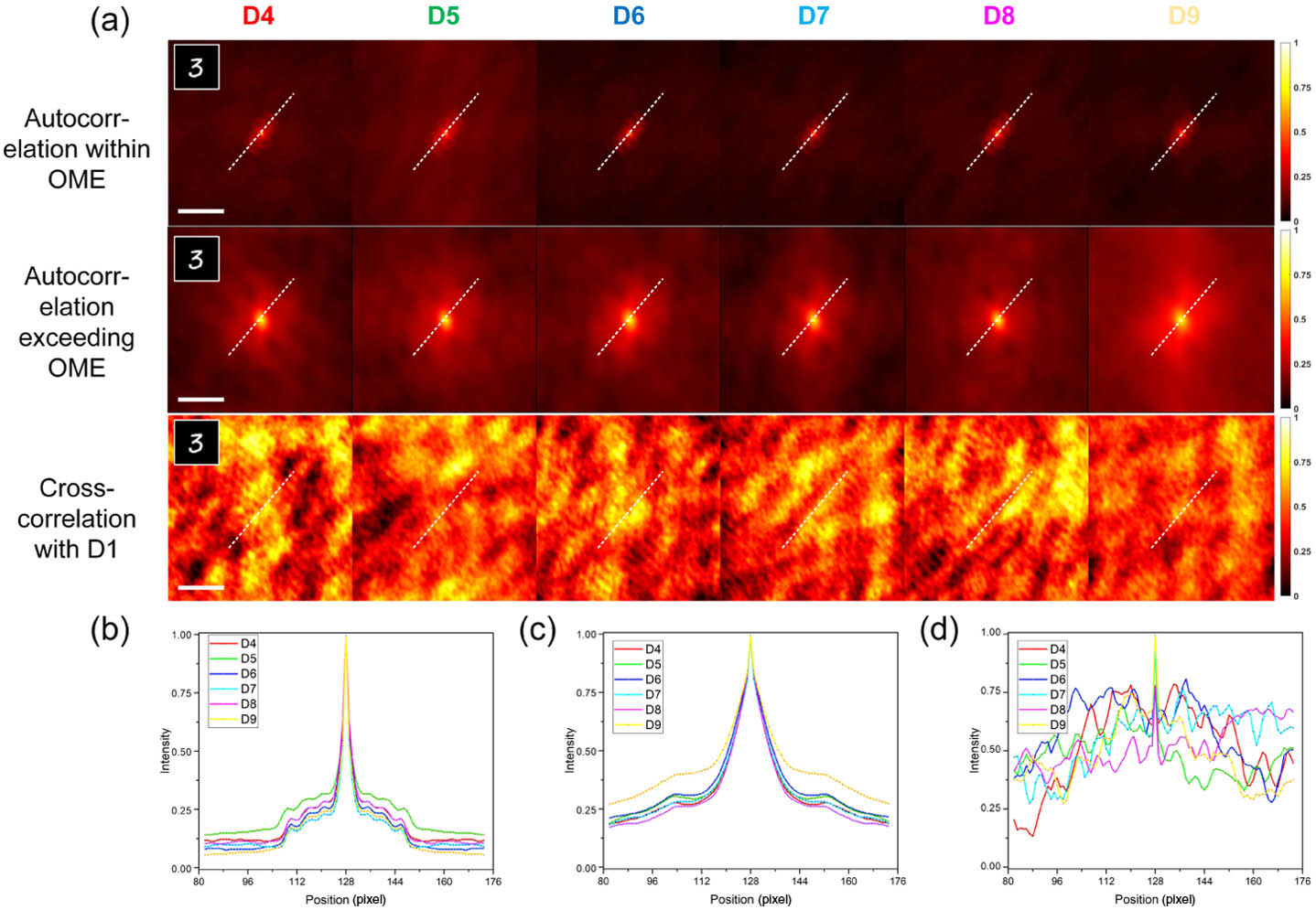
Fig. 1. Speckle statistical characteristics analysis of the same object corresponding to different testing diffusers. (a) First row and second row are the speckle autocorrelation of the object within or exceeding the OME range, the third row is the cross-correlation with D1, respectively. (b)–(d) Intensity values of the white dash lines in the first, second, and third rows of (a), respectively. The color bar represents the normalized intensity. Scale bars: 875.52 µm.

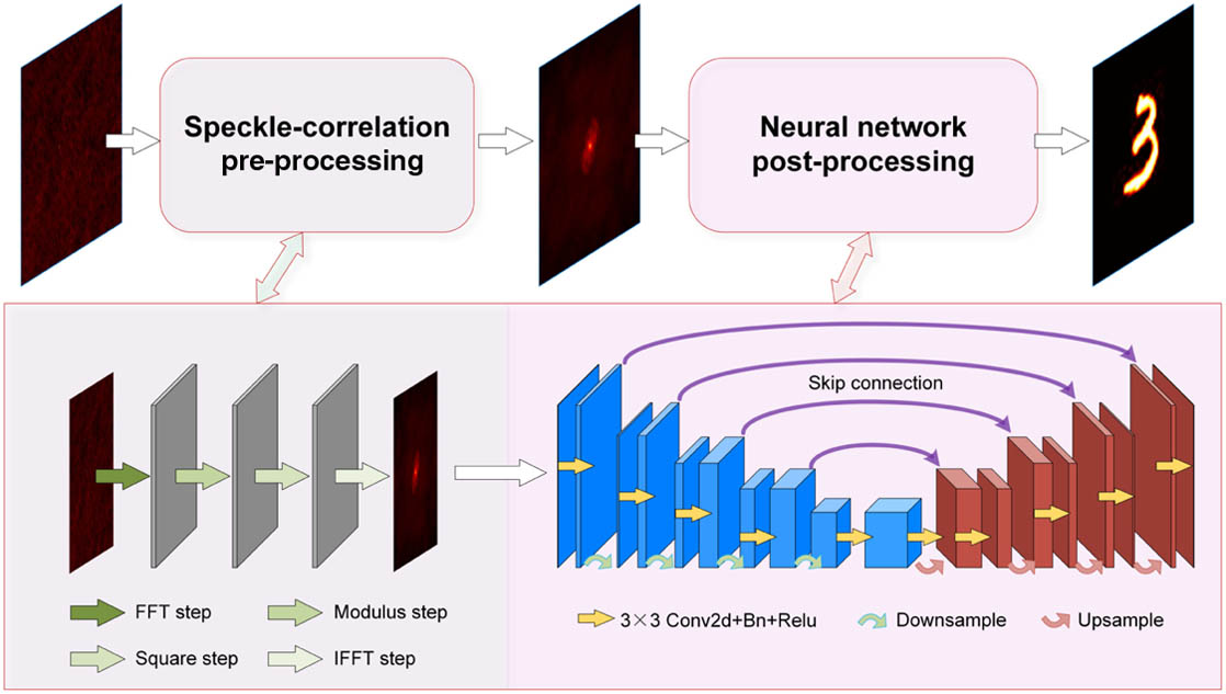
Fig. 2. Schematic of the physics-informed learning method for scalable scattering imaging.

Fig. 3. Experimental setup for the scalable imaging. Different diffusers are employed to obtain speckle patterns with different scattering scenes. The OME range of this system is also measured by calculating the cross-correlation coefficient [21]. See Appendix B for details.

Fig. 4. Testing results for generalization reconstruction of Group 1. Scale bars: 264.24 µm.

Fig. 5. Testing results for generalization reconstruction of Group 2. Scale bars: 264.24 µm.

Fig. 6. Testing results for generalization reconstruction of Group 3. Scale bars: 264.24 µm.

Fig. 7. Testing results for generalization reconstruction of Group 4. Scale bars: 820.8 µm.

Fig. 8. Generalization results for a single-character object with different scales and the scale of FOV is defined as the FOV/OME times. (a), (b) Results with different amounts of training diffusers, which are trained with one diffuser and three diffusers, respectively. (c) Reconstruction results with different scales and corresponding ground truth (GT).

Fig. 9. Comparison results without or with this pre-processing step for imaging through an unknown diffuser. Three ground glasses are selected as the training diffusers and another diffuser for testing.

Fig. 10. Results with different number of speckles via the physics-informed learning method. Three ground glasses are selected as the training diffusers and another diffuser for testing.

Fig. 11. Generalization results of imaging exceeding OME range with different complexity objects.

Table 1. Quantitative Evaluation Results of the Objects within OME

Table 2. Quantitative Evaluation Results of Objects Extending the FOV 1.2 Times

Table 3. Objective Indicators with Different Number of Speckles via the Physics-Informed Learning Method

Table 4. Objective Indicators Corresponding to Fig. 11