
Wang Zhang, Xiaorong Gao, Jinlong Li, Yu Zhang, Lin Luo. Three-Dimensional Surface Reconstruction of Rail Based on Two-Step Phase-Shift Method[J]. Laser & Optoelectronics Progress, 2022, 59(10): 1015003
- Laser & Optoelectronics Progress
- Vol. 59, Issue 10, 1015003 (2022)
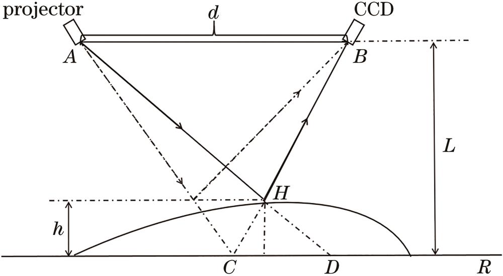
Fig. 1. Diagram of measuring optical path
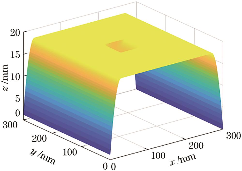
Fig. 2. Simulated 3D drawing of rail surface
Fig. 3. Standard sinusoidal fringe image. (a) Fringe image; (b) intensity distribution
Fig. 4. Sinusoidal fringe image with nonlinearity. (a) Fringe image; (b) intensity distribution
Fig. 5. Sinusoidal fringe after twice Hilbert transforms. (a) Intensity distribution; (b) filtered part
Fig. 6. Stoilov phase shift algorithm. (a) Reconstruction result; (b) reconstruction error
Fig. 7. Two-step phase-shift method without compensating phase error. (a) Reconstruction result; (b) reconstruction error
Fig. 8. Two-step phase-shift method with compensating phase error. (a) Reconstruction result; (b) reconstruction error
Fig. 9. Comparison of cross section of defect. (a) Stoilov phase shift algorithm; (b) two-step phase-shift method without compensation; (c) two-step phase-shift method with compensation
Fig. 10. Rail deformation grating fringes required by Stoilov algorithm
Fig. 11. Grating fringes obtained by the proposed method after twice Hilbert transforms
Fig. 12. Wrapped phase maps. (a) Wrapped phase map of Stoilov method; (b) wrapped phase map of proposed method
Fig. 13. Experimental results of three-dimensional profile restoration of rail side. (a) Reconstruction result of Stoilov method; (b) reconstruction result of proposed method
|
Table 1. Error comparison of reconstruction results

Set citation alerts for the article
Please enter your email address
© Copyright 2018-2021 | Chinese Laser Press. All Rights Reserved 沪ICP备15018463号-20