Polished Surface Defect Detection Based on Intelligent Surface Analysis

Zihao Li; Fengzhou Fang; Zhonghe Ren; Gaofeng Hou

doi:10.3788/LOP230868

Journals >Laser & Optoelectronics Progress >Volume 60 >Issue 24 >Page 2412006 > Article

Laser & Optoelectronics Progress
Vol. 60, Issue 24, 2412006 (2023)

Polished Surface Defect Detection Based on Intelligent Surface Analysis

Zihao Li^1、2, Fengzhou Fang^1、2、*, Zhonghe Ren^1、2, and Gaofeng Hou^1、2

Author Affiliations

¹State Key Laboratory of Precision Measuring Technology and Instrument, Tianjin University, Tianjin 300072, China

²Labotatory of Micro/Nano Manufacturing Technology (MNMT), Tianjin 300072, China

show less

DOI: 10.3788/LOP230868 Cite this Article Set citation alerts

Zihao Li, Fengzhou Fang, Zhonghe Ren, Gaofeng Hou. Polished Surface Defect Detection Based on Intelligent Surface Analysis[J]. Laser & Optoelectronics Progress, 2023, 60(24): 2412006 Copy Citation Text

show less

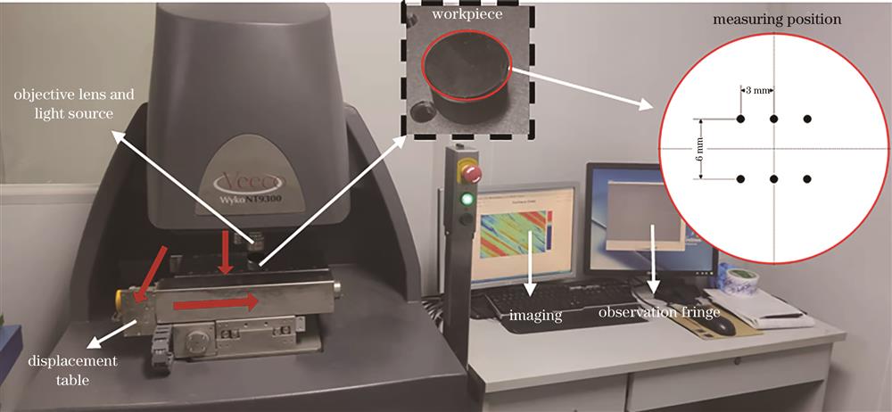
Fig. 1. Data collection system

Download full size

Fig. 2. Overall defect detection scheme based on surface analysis

Download full size

Fig. 3. Schematic diagram of intelligent profile analysis

Download full size

Fig. 4. Structure of FETN

Download full size

Fig. 5. Structure of FIFE block

Download full size

Fig. 6. Structure of cascaded receptive field enhancement defect detection model

Download full size

Fig. 7. Backbone network structure of defect detection model. (a) Backbone network structure; (b) comparison of defect characteristic receptive field

Download full size

Fig. 8. UPP-CLS dataset label distribution. (a) Label distribution before data balancing; (b) label distribution after data balancing

Download full size

Fig. 9. Results of FETN intelligent profile analysis and filtering

Download full size

Fig. 10. Height-to-width ratio statistics of dimension box in dataset

Download full size

Fig. 11. Comparison of the results between the proposed detection model and other mainstream detection models on the UPP-DET dataset. (a) Overall comparison; (b) partial comparison

Download full size

Fig. 12. Test results of defect detection model

Download full size

Parameter	UPP-CLS	UPP-DET
Batch size	8	4
Epoch	50	15
Initial learning rate	0.001	0.0002
Weight decay	‒	0.05
Optimizer	Adam	AdamW
Regularization	L2 weight decay	‒

Table 1. Basic parameters of the experiment

Vector ordering		SC	SE	Accuracy /%
L	C	SC	SE	Accuracy /%
‒	‒	‒	‒	75.18
√	‒	‒	‒	74.39
‒	√	‒	‒	78.07
‒	√	√	‒	78.24
‒	√	√	√	79.47

Table 2. Module performance analysis in the FIFE Block

Image branch backbone	FIFE	Accuracy /%	Sensitivity /%	FNR /%	TNR /%	Specificity /%
InceptionV3^［23］	‒	70.47	68.83	31.17	73.17	26.83
InceptionV3^［23］	√	74.44	71.23	28.77	77.70	22.30
ResNet-50^［21］	‒	75.18	73.64	26.36	77.88	22.12
ResNet-50^［21］	√	79.47	76.12	23.88	76.27	23.73
ResNet-101^［21］	‒	78.63	76.03	23.97	80.00	20.00
ResNet-101^［21］	√	83.98	79.68	20.32	83.21	16.79
MobileNetV3^［24］	‒	70.09	72.11	27.89	71.67	28.33
MobileNetV3^［24］	√	75.69	72.99	27.01	76.35	23.65
ResNext-50^［25］	‒	78.87	77.69	22.31	80.04	19.96
ResNext-50^［25］	√	82.21	77.15	22.85	84.76	15.24
EfficientNet-b2^［19］	‒	80.41	78.25	21.75	82.67	17.33
EfficientNet-b2^［19］	√	84.86	80.89	19.11	86.38	13.62
EfficientNet-b4^［19］	‒	82.11	79.97	20.03	84.64	15.36
EfficientNet-b4^［19］	√	85.36	81.49	18.51	87.72	12.28

Table 3. Comparative analysis of each model embedded in FIFE block

AD	Mixup	DC	mAP
—	—	—	0.697
√	—	—	0.721
√	√	—	0.729
√	√	√	0.740

Table 4. Performance analysis of each model embedded in FIFE block

Stage	Method	Backbone	MST	Scratch	Pit	mAP	FPS /（frame·s^-1）
One-stage	SSD300^［27］	VGG-16	‒	0.363	0.335	0.349	‒
	SSD512^［27］	VGG-16	‒	0.581	0.593	0.587	‒
	RetinaNet^［28］	ResNet-50	‒	0.775	0.749	0.762	‒
	Yolov3^［29］	DarkNet-53	‒	0.632	0.594	0.613	‒
	Yolov5	DarkNet-53	‒	0.816	0.782	0.799	‒
Two-stage	Faster R-CNN^［30］	ResNet-50	√	0.729	0.751	0.740	28.3
	Dynamic R-CNN^［31］	ResNet-50	√	0.816	0.798	0.807	24.9
	Cascade R-CNN^［18］	ResNet-50	√	0.815	0.822	0.819	22.7
	Proposed	EfficientNet-b4	√	0.867	0.840	0.854	21.1

Table 5. Comparison results between proposed model and other detection models

No.	$T_{I o U}$	mAP
Baseline	［0.5，0.6，0.7］	0.854
1	［0.2，0.6，0.7］	0.841
2	［0.3，0.6，0.7］	0.853
3	［0.4，0.6，0.7］	0.856
4	［0.4，0.5，0.6］	0.851
5	［0.4，0.5，0.7］	0.862
6	［0.4，0.5，0.8］	0.839

Table 6. IoU threshold analysis results at each stage of defect detection model detection head

Zihao Li, Fengzhou Fang, Zhonghe Ren, Gaofeng Hou. Polished Surface Defect Detection Based on Intelligent Surface Analysis[J]. Laser & Optoelectronics Progress, 2023, 60(24): 2412006

Download Citation

Set citation alerts for the article

Tools

Set citation alerts for the article

Save the article for my favorites

Paper Information