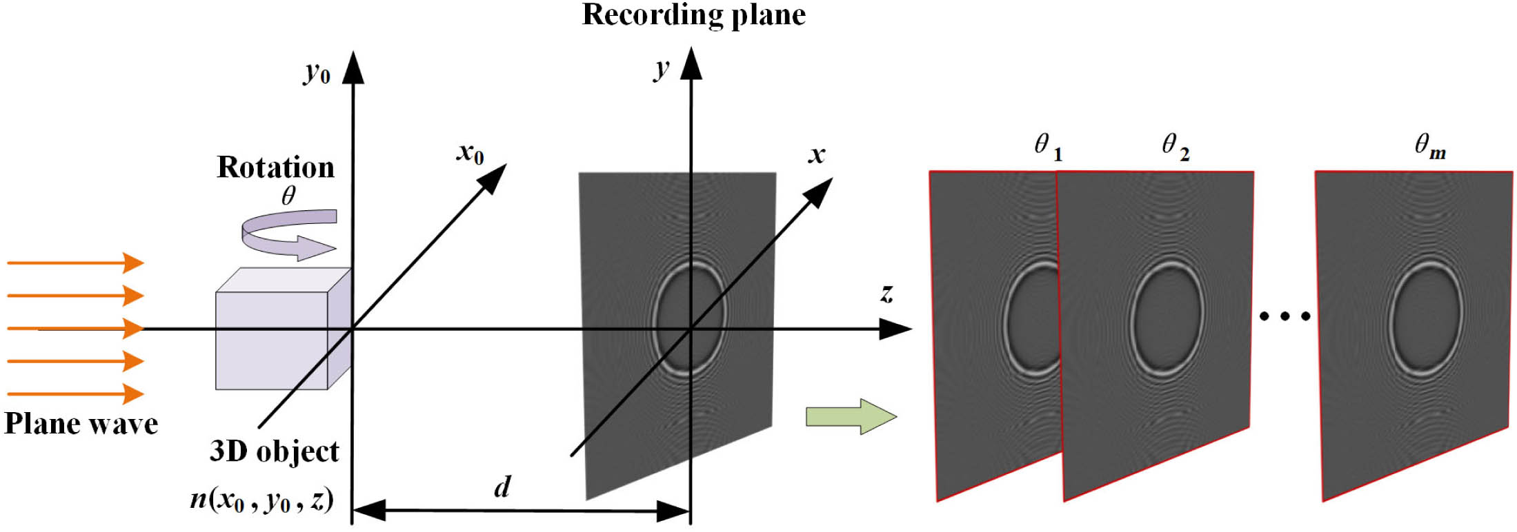
Fig. 1. Recording schematic of THz in-line digital hologram at different rotation angles.

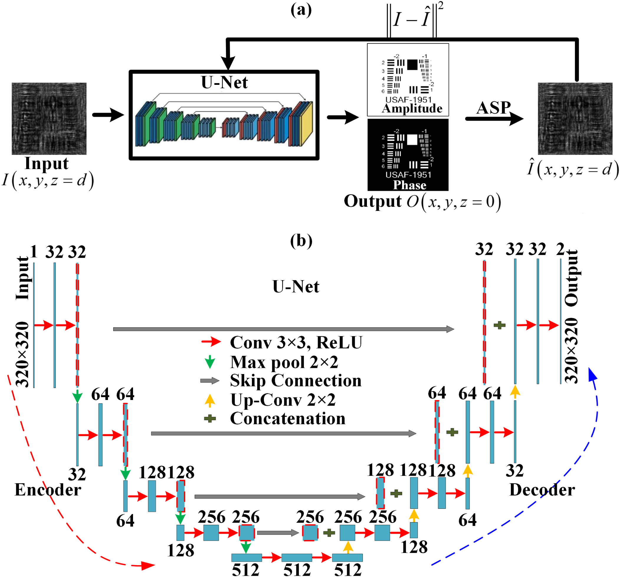
Fig. 2. Flowchart of the PhysenNet to reconstruct the in-line digital hologram. (a) Flowchart of the PhysenNet. (b) Schematic of the U-Net.

Fig. 3. Schematic of the setup of continuous-wave THz in-line digital holography. Off-axis parabolic mirrors, PM1 and PM2; rotational stage, RS.

Fig. 4. Comparison of the reconstructed results of the Siemens star and the cicada wing by different algorithms. (a) Photo of the Siemens star, (b) in-line hologram, (c) preprocessed normalized hologram, and (d)–(h) amplitude distributions by the backpropagation method, the ER method, the IDPR-RI method, the CCTV, and the PhysenNet, respectively.

Fig. 5. Comparison of the reconstructed results of the cicada wing by different algorithms. (a) Optical photo of the cicada wing; (b) normalized hologram; (c1)–(e1) and (c2)–(e2) amplitude and phase distributions by the IDPR-RI method, the CCTV, and the PhysenNet, respectively; and (f1) and (f2) amplitude and phase profiles of the white dashed line in (c1)–(e1) and (c2)–(e2).

Fig. 6. Comparison of the reconstructed results of a PS foam sphere by different algorithms at a single projection angle. (a) Optical photo of the sample, (b) normalized hologram, and (c1)–(g1) and (c2)–(g2) amplitude and phase distributions by the backpropagation method, the ER method, the IDPR-RI method, the CCTV, and the PhysenNet, respectively.

Fig. 7. Reconstructed refractive index distribution of a single PS foam sphere by the FBPP method. (a)–(c), (d)–(f), and (g)–(i) Refractive index profiles based on the DT-IDPR-RI, DT-CCTV, and DT-PhysenNet at x–z, y–z, and y–x cross sections, respectively. (j) Refractive index profiles of the white dotted line in (a), (d), and (g) (Visualization 1).

Fig. 8. Reconstructed refractive index distribution for two foam spheres. (a)–(c) Refractive index distributions at x–y and x–z (y1=2  mm, y2=3  mm) cross sections. (d) Volume rendering of the 3D refractive index distribution.

Table 1. Comparison of the Runtime for Different Phase Retrieval Algorithms