Continuous-wave terahertz in-line holographic diffraction tomography with the scattering fields reconstructed by a physics-enhanced deep neural network

Xiaoyu Jin; Jie Zhao; Dayong Wang; John J. Healy; Lu Rong; Yunxin Wang; Shufeng Lin

doi:10.1364/PRJ.493902

Abstract

Diffraction tomography is a promising, quantitative, and nondestructive three-dimensional (3D) imaging method that enables us to obtain the complex refractive index distribution of a sample. The acquisition of the scattered fields under the different illumination angles is a key issue, where the complex scattered fields need to be retrieved. Presently, in order to develop terahertz (THz) diffraction tomography, the advanced acquisition of the scattered fields is desired. In this paper, a THz in-line digital holographic diffraction tomography (THz-IDHDT) is proposed with an extremely compact optical configuration and implemented for the first time, to the best of our knowledge. A learning-based phase retrieval algorithm by combining the physical model and the convolution neural networks, named the physics-enhanced deep neural network (PhysenNet), is applied to reconstruct the THz in-line digital hologram, and obtain the complex amplitude distribution of the sample with high fidelity. The advantages of the PhysenNet are that there is no need for pretraining by using a large set of labeled data, and it can also work for thick samples. Experimentally with a continuous-wave THz laser, the PhysenNet is first demonstrated by using the thin samples and exhibits superiority in terms of imaging quality. More importantly, with regard to the thick samples, PhysenNet still works well, and can offer 2D complex scattered fields for diffraction tomography. Furthermore, the 3D refractive index maps of two types of foam sphere samples are successfully reconstructed by the proposed method. For a single foam sphere, the relative error of the average refractive index value is only 0.17%, compared to the commercial THz time-domain spectroscopy system. This demonstrates the feasibility and high accuracy of the THz-IDHDT, and the idea can be applied to other wavebands as well.

1. INTRODUCTION

Terahertz (THz) waves, ranging from 0.1 to 10 THz, are located between infrared and microwave in electromagnetic waves. They have various special properties, such as high penetration through nonmetallic and nonpolar materials, low photon energy, and fingerprint spectrum of biological and medical materials. Therefore, THz waves are widely used in biomedical fields [1], nondestructive testing [2], and three-dimensional (3D) imaging [3,4], e.g., complementary medical diagnosis of melanoma and brain gliomas [5], nondestructive defect testing of aircraft composite materials from mechanical or heat damage [6], and pigment identification in cultural relic restoration [7].

Remarkably, with the development of the elements manufactured by using the new technologies, such as additive manufacturing and photolithography, the requirements for detecting the internal 3D structure and the defects are increasing [8]. Tomography is an effective method for 3D imaging, among which computed tomography and diffraction tomography are the most commonly known. Computed tomography based on the geometrical straight-line model for the propagation of radiation is suitable for shorter wavelengths, such as X-ray and electron beam. Although THz computed tomography has also been well developed, the reconstructed results could suffer from severe blurring and distortion, for a sample with high refractive index contrast, complex structure, or large optical path difference, because of the large wavelength of THz waves [3]. The diffraction tomography that takes the diffraction and scattering into account is available for a wider range of wavelengths, and also for THz waves. In THz diffraction tomography, it is essential that the complex field of the projection data is acquired accurately and efficiently; the developed methods include the THz time-domain spectroscopy (THz-TDS) system [9] and THz off-axis digital holography [10]. The THz-TDS system provides the electric field of the hyperspectral information by optical delay line [11]. Due to the requirements of scanning, it is hard to obtain the amplitude and phase distribution of the sample in a fast and full-field way, and the resolution is also restricted by the size of the scanning beam. Although the electro-optic sampling is a full-field imaging method based on the THz-TDS system that accelerates the detection of two-dimensional (2D) THz electric field, it is limited by the modulation efficiency of the electro-optic crystal [9]. THz off-axis digital holography is another quantitative phase-contrast imaging (QPI) technology [12], but its additional reference beam increases the complexity of the optical systems and reduces the utilization of spatial bandwidth.

Due to the more compact optical configuration, THz in-line digital holography [13] is a more promising method for acquiring projection data. However, the twin-image problem and the limitation of sample size obstruct its application. Fortunately, the phase-shifting and the numerical iterative approaches have been developed for eliminating the twin image. Being different from the complicated optical configuration of the phase-shifting method, the numerical iterative approaches do not require additional hardware devices, and they can eliminate or suppress the twin image through the known physical constraints. The traditional numerical approach is applying the finite-support constraint at the object plane or a sequence of intensity pattern constraints at different recording planes. Recently, compressive sensing [14], sparse optimization [15,16], iterative denoising phase retrieval (IDPR) [17], and multiplane phase retrieval [18] methods have been developed to overcome the twin-image problem. In addition to the twin-image problem, the resolution is also significant for the THz in-line digital holography. To enhance or improve the resolution, the synthetic aperture [16] and extrapolation [19] methods have also been explored. Although the transport-of-intensity equation is also an in-line configuration [20,21], two intensity images (in focus and defocus) need to be recorded at least.

Sign up for Photonics Research TOC. Get the latest issue of Photonics Research delivered right to you！Sign up now

In the visible light, deep learning (DL) exhibits huge potential in various areas of computational imaging, such as computational ghost imaging, digital holography, imaging through scattering media [22], and diffraction tomography [23]. The phase retrieval methods based on the convolution neural networks (CNNs) are also proposed to solve the twin-image problem. Benefiting from the excellent fitting power of the CNNs, it enables further improvement of the reconstruction quality [24]. According to the training process, the CNNs-based phase retrieval methods are categorized in two ways: one is an end-to-end neural network, which requires a large amount of labeled data to pretrain the CNNs [25,26], and the other is a physics-enhanced deep neural network combining a physical model with the CNNs, which requires only a small amount of measurement data to train the CNNs [27,28], e.g., in single-frame [27], two-frame [28], and dual-wavelength [29] in-line digital holography. In the THz band, the combination of the CNNs and THz imaging has also attracted increasing attention from researchers in the past few years, and the existing studies are mainly focused on improving the resolution of the THz intensity imaging [30,31]. Although the complex CNNs-based methods have also been presented to simultaneously improve the resolution of the amplitude and phase images [32], they are all end-to-end methods. More ominously, with the lack of available devices, it is difficult to achieve an enormous amount of labeled data for pretraining, and this is an important factor that limits the combination of the CNNs and various THz imaging methods. Actually, the CNNs-based methods are needed even more in the THz band. First, both the THz sources and detectors are currently in the early stages of development, and their stability and signal-to-noise ratios are relatively low. Thus, algorithms of THz imaging with better performance and robustness are increasingly required, for which the CNNs-based methods are a possible solution. Second, the pixel numbers of detectors in the THz band are significantly less than those in the visible light [33], so the CNNs-based methods provide a more efficient pretraining process as well.

In this paper, THz in-line digital holographic diffraction tomography (THz-IDHDT) was first proposed for 3D imaging of the sample. In order to obtain the complex distribution of the projection data with high fidelity, a learning-based phase retrieval algorithm was implemented to reconstruct the in-line digital holograms by combining the physical model and the CNNs (PhysenNet). The main advantage of the PhysenNet is that there is no need for tens of thousands of labeled data for pretraining, and it can automatically optimize the network parameters. Besides, it can also work for thick samples, for which the traditional phase retrieval methods usually will not give the results with reasonable quality. To the best of our knowledge, it is the first time that the PhysenNet is applied in the THz in-line digital holography. An experimental setup was built based on a continuous-wave THz source with a frequency of 2.52 THz, where the Gabor in-line digital holograms were recorded by a pyroelectric detector. In the experiments, the feasibility of the PhysenNet was verified using both the thin and thick samples, respectively. It is necessary to record at least several dozens of holograms of the projection data in THz-IDHDT, but, at this point, it is relatively time-consuming to use the general one-to-one training process of the PhysenNet, i.e., one hologram corresponds to one PhysenNet. To decrease the reconstruction time of the PhysenNet, a joint training process is proposed; i.e., all the recorded digital holograms are used to train a PhysenNet. Subsequently, the 3D refractive index distribution of both the single and two glued foam spheres was also successfully reconstructed by the THz-IDHDT. Compared with the average refractive index value measured by the THz-TDS system, the relative error of the proposed method is only 0.17% for a single foam sphere. Thus, it is confirmed that the proposed THz-IDHDT provides an accurate quantification of the refractive index distribution of the sample in 3D.

This paper is organized as follows. In Section 2, the principles of THz in-line digital holographic diffraction tomography are introduced, including the pipeline of the PhysenNet for the phase retrieval and the 3D reconstruction of THz diffraction tomography. In Section 3, the 2D amplitude and the phase distributions under a single projection angle reconstructed by PhysenNet are presented, and then the 3D refractive index distribution is reconstructed by filtered backpropagation (FBPP) algorithm using the retrieved scattering fields. Finally, summaries are drawn in Section 4.

2. PRINCIPLES

A. Recording the Scattered Fields Based on THz In-Line Digital Holography

The recording principle of the THz in-line digital holography is shown in Fig. 1, which is Gabor type. First, we assume that a plane wave from a coherent THz source with a wavelength of $λ$ is incident on a 3D object, and the transmitted wave field of the object at a rotation angle of $θ_{m}$ can be expressed as $U_{0} (x_{0}, y_{0}; θ_{m}) = 1 + Δ t (x_{0}, y_{0}; θ_{m}), m = 1, 2, \dots, M,$ (1)where $(x_{0}, y_{0})$ are the spatial coordinates at object plane, the constant “1” in Eq. (1) represents the nondiffracted light of the transmitted light, which is regarded as the reference beam, and $Δ t (x_{0}, y_{0}; θ_{m})$ in Eq. (1) is the diffracted light modulated by the object, which is regarded as the object beam. When the reference beam and the object beam propagate to the recording plane, they interfere with each other, whose intensity distribution forms the hologram as $I (x, y; θ_{m}) = 1 + {| Δ T |}^{2} + Δ T + Δ T^{*},$ (2)where $Δ T$ and $Δ T^{*}$ represent the object beam and its conjugate term on the hologram plane, respectively. Then, by rotating the object, a series of in-line digital holograms were recorded using the THz array detector at the different rotation angles (range from 0° to 360°). Because the object beam and the reference beam share the same optical path, the reconstruction quality was seriously degraded by the twin image. In order to remove the twin image, the PhysenNet is introduced.

Recording schematic of THz in-line digital hologram at different rotation angles.

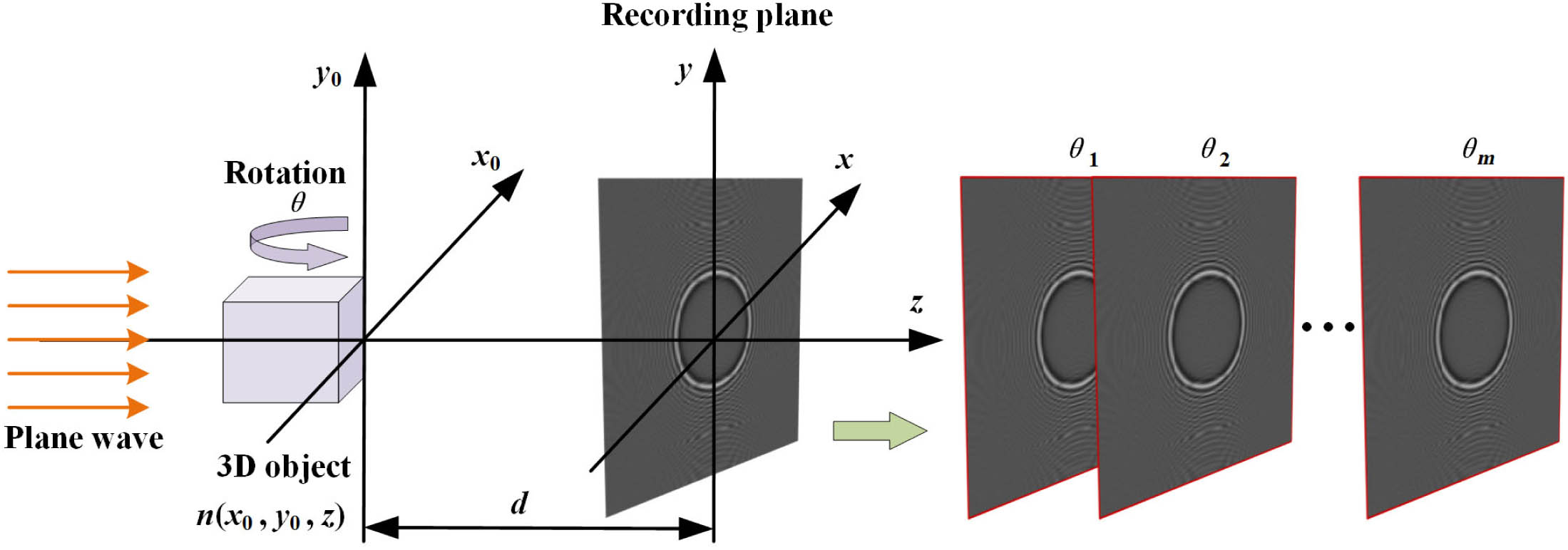
Figure 1.Recording schematic of THz in-line digital hologram at different rotation angles.

B. PhysenNet for Reconstructing the Scattered Fields

The reconstruction of the THz in-line digital holography by using the PhysenNet is shown in Fig. 2(a); it consists of two main components: a neural network model and a diffraction propagation model. By combining the two models, the process of its phase retrieval can be roughly divided into three steps. Step 1: the preprocessed normalized hologram is first fed into the neural network, and the output of the neural network is assumed to be the amplitude and phase distribution in the object plane. Step 2: the predicted complex field is forward propagated to the recording plane to obtain the estimated intensity distribution of the hologram. Step 3: the loss is calculated between the estimated hologram and the experimentally recorded hologram; then, the weights of the neural network are updated according to the loss. Steps 1–3 are repeated for training the neural network. By multiple iterations, the complex scattered field at a certain illumination angle can be reconstructed with high fidelity.

Figure 2.Flowchart of the PhysenNet to reconstruct the in-line digital hologram. (a) Flowchart of the PhysenNet. (b) Schematic of the U-Net.

In our algorithm, U-Net [34], a CNN is employed as the neural network model, which has been widely applied in various fields of computational imaging. The detailed schematic of the U-Net is presented in Fig. 2(b); its architecture includes the convolution layer, max pooling layer, transposed convolution layer, concatenation, and skip connection. The U-Net is an encoder–decoder architecture; the left side can be regarded as the encoder, which is responsible for feature extraction of the input data, and the right side can be regarded as the decoder, which is responsible for recovering the image. In the decoder, the skip connection is extremely important; it can fuse the deep and shallow features as well as solving the vanishing gradient problem.

First, the normalized in-line digital hologram is adopted as the input of the U-Net, and the output of the U-Net is assumed to be the complex amplitude distribution ${\hat{O}}_{z = 0} (x_{0}, y_{0}; θ_{m})$ in the object plane, ${\hat{O}}_{z = 0} (x_{0}, y_{0}; θ_{m}) = f [I (x, y; θ_{m}), w],$ (3)where $f$ and $w$ are the designed U-Net and the corresponding weight, respectively.

Then, it is propagated to the recording plane by the angular spectrum propagation (ASP) method [35], which can be expressed as $U_{z = d} (x, y; θ_{m}) = F^{- 1} {F {{\hat{O}}_{z = 0} (x_{0}, y_{0}; θ_{m})} H_{z = d} (f_{x}, f_{y})},$ (4)where $H_{z = d} (f_{x}, f_{y}) = {\begin{cases} \exp [j k_{0} d \sqrt{1 - {(λ f_{x})}^{2} - {(λ f_{y})}^{2}}], & f_{x}^{2} + f_{y}^{2} < \frac{1}{λ^{2}} \\ 0, & else \end{cases} .$ (5) $F$ and $F^{- 1}$ represent the Fourier transform and inverse Fourier transform, $H_{z = d} (f_{x}, f_{y})$ is the transfer function, $(f_{x}, f_{y})$ are the coordinates of the spatial spectrum in the recording plane, $λ$ is the wavelength, $k_{0} = 2 π / λ$ is the wave number, and $d$ is the distance from the object plane to the recording plane. And the intensity distribution of the estimated hologram on the recording plane can be written as ${\hat{I}}_{z = d} (x, y; θ_{m}) = {| U_{z = d} (x, y; θ_{m}) |}^{2} .$ (6)

With the estimated hologram and the experimentally recorded hologram, the loss function of the PhysenNet can be given as $L (x, y; θ_{m}) = \underset{w}{\arg \min} {‖ I (x, y; θ_{m}) - \hat{I} (x, y; θ_{m}) ‖}_{2}^{2} .$ (7)

From the above loss function, it is revealed that the proposed method does not require the ideal amplitude and phase distribution of the sample to be known. Instead, it is a combination of a physical model and CNNs that allows the CNNs to indirectly capture the mapping relationship between the experimentally recorded hologram and the complex amplitude distribution of the sample. When the weight parameters of the CNNs are optimized, the amplitude ${\hat{A}}_{z = 0}$ and phase ${\hat{φ}}_{z = 0}$ of the sample without the twin image can be denoted as ${\hat{A}}_{z = 0} (x_{0}, y_{0}; θ_{m}) = abs {{\hat{O}}_{z = 0} (x_{0}, y_{0}; θ_{m})},$ (8) ${\hat{φ}}_{z = 0} (x_{0}, y_{0}; θ_{m}) = angle {{\hat{O}}_{z = 0} (x_{0}, y_{0}; θ_{m})},$ (9)where $abs {\cdot}$ and $angle {\cdot}$ are the operators to calculate the amplitude and phase of complex numbers, respectively.

In this paper, our models were implemented and tested using the TensorFlow Framework in a high-performance laptop with an NVIDIA RTX 3070 graphics card and an i9-CPU. The Adam optimizer was adopted to optimize the weight parameters [36], and the learning rate gradually decays as the training proceeds. Moreover, to avoid the overfitting problem, a uniformly distributed noise between 0 and 0.02 was added to the input hologram at each 500 iterations. In general, it has converged around 10,000 epochs. When the training of the PhysenNet is complete, the added noise is removed from the input hologram and the estimated amplitude and phase distributions of the sample are calculated according to Eqs. (8) and (9).

C. Three-Dimensional Reconstruction Algorithm of THz Diffraction Tomography

After reconstructing the transmitted wave field ${\hat{O}}_{z = 0} (x_{0}, y_{0}; θ_{m})$ of the sample at all rotation angles using PhysenNet, the weak scattering approximation of the transmitted wave field is required. The Rytov approximation does not limit the size of the sample [37], but only needs to satisfy that the phase change of the sample is sufficiently small. Therefore, the Rytov approximation is carried out, and the scattered field $O_{s} (x_{0}, y_{0}; θ_{m})$ can be expressed as $O_{s} (x_{0}, y_{0}; θ_{m}) \approx O_{in} (x_{0}, y_{0}) \ln [{\hat{O}}_{z = 0} (x_{0}, y_{0}; θ_{m}) / O_{in} (x_{0}, y_{0})],$ (10)where $O_{in} (x_{0}, y_{0})$ is the incident plane wave. Once the Rytov approximation of the transmitted wave fields at all rotation angles is completed, the 3D reconstruction of the sample can be performed using the diffraction tomography theory.

The adopted FBPP algorithm is employed as a spatial domain reconstruction algorithm of the diffraction tomography [38], which does not require the frequency domain interpolation and can effectively avoid the error-prone frequency interpolation in the frequency domain interpolation algorithm. Therefore, the FBPP algorithm is widely used in diffraction tomography for object rotation configurations. The calculation process of the FBPP algorithm is shown in Eq. (11): $f (x_{0}, y_{0}, z_{0}) = \frac{- i k_{0}}{4 π^{2}} \int_{0}^{2 π} \int_{- k_{0}}^{k_{0}} \int_{- k_{0}}^{k_{0}} | k_{D_{x_{0}}} | {\tilde{O}}_{s} (k_{D_{x_{0}}}, k_{D y_{0}}; θ_{m}) \times \exp [i z_{θ_{m}} (\sqrt{k_{0}^{2} - k_{D x_{0}}^{2} - k_{D y_{0}}^{2}} - k_{0})] \times \exp [i (k_{D x_{0}} x_{θ_{m}} + k_{D y} y_{θ_{m}})] d k_{D x_{0}} d k_{D y_{0}} d θ_{m},$ (11)where $x_{θ_{m}} = x_{0} \cos θ_{m} + z_{0} \sin θ_{m},$ (12) $y_{θ_{m}} = y_{0},$ (13) $z_{θ_{m}} = - x_{0} \sin θ_{m} + z_{0} \cos θ_{m} .$ (14)

It is seen that the FBPP algorithm can be composed of two steps: the first step is to filter and backpropagate the 2D scattering field. The second step is to stack the backpropagation results at all rotation angles in the three dimensions to obtain the scattering potential $f$ of the measured sample. Finally, the scattering potential distribution can be converted into the refractive index distribution by using Eq. (15), namely $n (x_{0}, y_{0}, z_{0}) = n_{0} \sqrt{\frac{f (x_{0}, y_{0}, z_{0})}{k_{0}^{2}} + 1},$ (15)where $n_{0}$ and $k_{0}$ are the refractive index distribution of the homogeneous medium around the sample and the corresponding wave number.

3. EXPERIMENTAL RESULTS

A. Experimental Setup

The experimental apparatus of the in-line digital holography was built using a continuous-wave THz source as shown in Fig. 3. The THz source is an optical pumped far-IR gas laser (295-FIRL-HP; Edinburgh Instruments Ltd., UK) with a central wavelength of 118.83 μm (2.52 THz) and a maximum power of 500 mW. First, the emitted THz beam is expanded and collimated by two off-axis parabolic mirrors (PM1, $f_{1} = 50.8 mm$ ; PM2, $f_{2} = 152.4 mm$ ); the beam size becomes two times bigger than the original one. The final spot diameter of the illumination beam is approximately 25 mm. The expanded THz beam propagates for a small distance, and then illuminates the sample. The diffracted light modulated by the object as object beam and the nondiffracted light as the reference beam both propagate to the recording plane along the same optical path. Finally, the in-line holograms are recorded by a pyroelectric detector (Pyrocam III, Ophir Spiricon). It has $320 \times 320$ pixels with $80 μm \times 80 μm$ pixel pitch and 50 Hz chopping frequency. Here, 500 frames of the holograms are recorded and accumulated via Gaussian fitting to improve the contrast of the digital hologram. In order to obtain the projection data of the sample under different illumination angles, a rotational stage (PRMTZ8/M; Thorlabs Inc., USA) for rotating the sample is added to the original optical path, as shown in the blue dashed area in Fig. 3. Thus, by rotating the sample, the in-line digital holograms of the sample at the different rotation angles can be achieved.

Figure 3.Schematic of the setup of continuous-wave THz in-line digital holography. Off-axis parabolic mirrors, PM1 and PM2; rotational stage, RS.

B. Digital Holographic Reconstruction under a Single Projection Angle

To demonstrate the effectiveness of the PhysenNet, the thin and thick samples are both tested at the rotation angle of 0°, respectively. In our experiments, the PhysenNet is compared with other phase retrieval algorithms, including the backpropagation method based on the ASP, the error reduction (ER) method [39], the iterative denoising phase retrieval method based on real and imaginary parts (IDPR-RI) [17], and the complex constrained total variation regularization (CCTV) method [40].

1. Thin Samples

First, a binary Siemens star resolution plate and a forewing of cicada were tested as shown in Fig. 4. The Siemens star is made by fabricating gold-film bars on a silicon substrate. At a frequency of 2.52 THz, silicon has a high transmittance with a refractive index of 3.4175. To quantitatively evaluate the experimental results reconstructed by different methods, a blind image quality assessment model named the natural image quality evaluator (NIQE) is adopted [41]. The NIQE is a kind of the reference-free image evaluation function, so only the recovered image is required as the input data, and the smaller NIQE values represent better quality of the experimental results. Figures 4(b) and 4(c) are the recorded hologram and the corresponding normalized hologram, where the recording distance of the hologram is about 32.5 mm. Figures 4(d)–4(h) are the amplitude distributions reconstructed by the backpropagation method, the ER method, the IDPR-RI method, the CCTV, and the proposed PhysenNet. It can be estimated that the opaque parts of the Siemens star occupy about 32% of the illumination area. The opaque parts of the Siemens star are treated as the effective area of the sample, which has exceeded the sparse requirement as stated in Ref. [42]. Therefore, the ER method is ineffective for this sample. On the contrary, the IDPR-RI method, the CCTV, and the PhysenNet can not only reduce the twin image, but also relax the limitation of the sample size in the Gabor in-line digital holography to a certain extent. The IDPR-RI method treats the twin image as noise superimposed in the object plane, and then the denoising process embedded in each iteration is applied to the real and imaginary parts of the object field, respectively. Therefore, it is also enabled to obtain better reconstruction results. The CCTV adopts the complex constrained total variation regularization instead of real part total variation regularization, so that the twin image is also suppressed. The reconstructed amplitudes and phases by the PhysenNet have the lower NIQE values and also have sharper edges. More obviously, the background region reconstructed by the PhysenNet has less noise interference, which demonstrates the advantages of the proposed method in terms of the twin-image suppression and noise reduction. Similarly, from the reconstructed results of the cicada wing in Fig. 5, it is also seen that the amplitude and phase distributions reconstructed by the PhysenNet have the best quality; it is demonstrated from its smaller NIQE value. From Figs. 5(f1) and 5(f2), the amplitude and the phase distributions reconstructed by the PhysenNet have better contrast between the wing membrane and the wing veins, which implies better image resolution. The size of the clearly observed vein is about 170 μm. It is noted that here the U-Net establishes the mapping relation between the intensity of the hologram and the complex amplitude distribution of the object. Only the forward diffraction propagation model is used to produce estimated measurements to drive the training of the CNNs so that it automatically optimizes the weights and bias of the U-Net to suppress the twin image better. It is mainly beneficial from the interplay between a handcrafted network structure and a physical diffraction propagation model.

Figure 4.Comparison of the reconstructed results of the Siemens star and the cicada wing by different algorithms. (a) Photo of the Siemens star, (b) in-line hologram, (c) preprocessed normalized hologram, and (d)–(h) amplitude distributions by the backpropagation method, the ER method, the IDPR-RI method, the CCTV, and the PhysenNet, respectively.

Figure 5.Comparison of the reconstructed results of the cicada wing by different algorithms. (a) Optical photo of the cicada wing; (b) normalized hologram; (c1)–(e1) and (c2)–(e2) amplitude and phase distributions by the IDPR-RI method, the CCTV, and the PhysenNet, respectively; and (f1) and (f2) amplitude and phase profiles of the white dashed line in (c1)–(e1) and (c2)–(e2).

In addition to the above-mentioned reconstruction quality, there are two aspects to discuss below. The first aspect is the experimental resolution, which can be revealed by using the Siemens star sample, given by the following equation: $c = r \times \sin α,$ (16)where $r$ is the distance from the center of the Siemens star to the distinguishable position, and $α = 7.5 °$ . The inset figures of Figs. 4(f)–4(h) are the zoomed-in results of the red dashed area, where the one-dimensional (1D) amplitude distributions at the white solid line are shown. From Figs. 4(f)–4(h), the distances from the white solid line to the center of the Siemens star are calculated as $r_{IDPR-RI} \approx 1303 μm$ , $r_{CCTV} \approx 1530 μm$ , and $r_{PhysenNet} \approx 1270 μm$ ; thus the lateral resolution of the IDPR-RI, the CCTV, and the PhysenNet can be calculated as $c_{IDPR-RI} \approx 170.1 μm$ , $c_{CCTV} \approx 199.7 μm$ , and $c_{PhysenNet} \approx 165.7 μm$ subsequently with Eq. (16). According to Abbe’s diffraction limit, the theoretical resolution equals $ρ = 0.5 λ / \sin θ_{\max}$ , where $θ_{\max}$ is the maximum diffraction angle. When the recording distance is $d \approx 32.5 mm$ , the theoretical resolution is $ρ \approx 161.2 μm$ . Therefore, the experimental results reconstructed by the PhysenNet are more in agreement with the theoretical value.

The second aspect is that for the phase retrieval algorithms, the time consumption of the algorithm is also a more important factor in some applications, which are discussed below for the different algorithms. For a fair comparison, the stopping conditions of the different phase retrieval algorithms are the same; i.e., the mean square error (MSE) between the reconstructed amplitude of two adjacent iterations is less than $10^{- 4}$ . Through several tests, the time consumption of the different algorithms is shown in Table 1. As illustrated from the table, PhysenNet takes the most time. However, with the GPU acceleration, the PhysenNet requires only about 8 min, and the computing speed has increased by nearly 53 times. This is one of the drawbacks of the neural network-based computational imaging methods. The prediction time in the order of minutes will not be enough to meet some dynamic applications. The computational time needed to be improved. It is worthwhile to note that for the applications where almost a real-time reconstruction is required, it is possible to make the PhysenNet have faster reconstruction. It can be realized by adopting the joint training process, e.g., using some of the recorded data for the training of the PhysenNet. Then it will largely reduce the computational time.Table 1.

Comparison of the Runtime for Different Phase Retrieval Algorithms

Algorithms	Platform	Iterations	Time
ER	CPU	200	$\sim 6 s$
IDPR-RI	CPU	50	$\sim 42 s$
CCTV	CPU	500	$\sim 68 s$
PhysenNet	CPU	10,000	$\sim 430 \min$
PhysenNet	CPU + GPU	10,000	$\sim 8 \min$

2. Thick Samples

For the thicker samples, a single polystyrene (PS) foam sphere is tested by the in-line digital holography in the experiment. The adopted PS foam sphere is shown in Fig. 6(a) with a diameter of about 6.58 mm and a refractive index of about 1.0169 (which is measured using THz-TDS). Figure 6(b) is the normalized hologram. The reconstructed amplitude and phase distributions by the backpropagation method, the ER method, the IDPR-RI method, the CCTV, and the PhysenNet are illustrated in Figs. 6(c1)–6(g1) and 6(c2)–6(g2), respectively. It can be revealed that neither the ER method nor the IDPR-RI method can effectively reconstruct the amplitude and phase distribution of the PS foam sphere. This is because the above two methods use the iterative strategy of the positive absorption constraint on the object plane, which only works for thin samples. However, for thicker samples, the positive absorption constraint becomes invalid, leading to the failure of the reconstruction. In contrast, both the CCTV and PhysenNet are gradient descent-based optimization methods. Among them, the CCTV quantifies the error between the estimated hologram and the actual measured hologram by a loss function, and accordingly updates the current estimate based on the gradient of the error. The PhysenNet first uses the gradient of the error to optimize the parameters of the CNNs for the purpose of updating the current estimate. Therefore, when the positive absorption constraint is invalidated, the CCTV and PhysenNet are still effective. Due to the robust fitting capability of the CNNs, PhysenNet has improved performance. The complex amplitude distribution reconstructed by PhysenNet has higher quality and fidelity compared with CCTV, and the threads of the support rod in the reconstructed amplitude are clearly distinguished, as demonstrated in Fig. 6(g1), which means higher image resolution. In order to evaluate quantificationally, two rectangle regions are chosen in Figs. 6(f2) and 6(g2), and the root mean square error (RMSE) values are calculated as 0.1158 and 0.0361, respectively. This shows that the background of the results obtained by PhysenNet is more even.

Figure 6.Comparison of the reconstructed results of a PS foam sphere by different algorithms at a single projection angle. (a) Optical photo of the sample, (b) normalized hologram, and (c1)–(g1) and (c2)–(g2) amplitude and phase distributions by the backpropagation method, the ER method, the IDPR-RI method, the CCTV, and the PhysenNet, respectively.

C. Three-Dimensional Reconstruction of the Refractive Index Distribution

Regardless of the thin or thick samples, their amplitude and phase distributions reconstructed by the phase retrieval algorithms or the other THz QPI method are the integration of the absorption coefficient and refractive index of the sample in the illumination direction, respectively, which only reflect part of the 3D structure distribution of the sample at a certain illumination angle. To obtain the 3D information of the sample, a 3D imaging method combining the in-line digital holography with diffraction tomography was implemented in the THz band for the first time, to the best of our knowledge. Its reconstruction process consists of two steps. First, using the PhysenNet, the complex amplitude distributions of the sample at various rotation angles were reconstructed in the in-line digital holography; it provides the projection data for the reconstruction of the diffraction tomography. For the traditional one-to-one training mode, i.e., one PhysenNet corresponds to one digital hologram, according to the Table 1, with GPU acceleration, 8 min is required for one digital hologram. There are in total 72 digital holograms; then it will take about 576 min. Here, a joint training procedure is proposed, where all the recorded digital holograms are used to train a PhysenNet, and the training time is largely reduced to 40 min. The effectiveness of the joint training process is because its complex amplitudes at adjacent rotation angles have partial overlap for the same sample. Thus, by utilizing this redundancy information, a PhysenNet can be trained rapidly without using a large amount of training data. Then, the 3D complex refractive index distribution of the sample was obtained through the FBPP method based on the Rytov approximation.

In the experiments, the sample was rotated gradually by 360° at angular intervals of 5°; thus 72 in-line holograms with the object were recorded successively, followed by the illumination beam without the object. Figure 7 shows the reconstructed refractive index distribution by the FBPP method based on IDPR-RI, CCTV, and PhysenNet (named as DT-IDPR-RI, DT-CCTV, and DT-PhysenNet), in which Figs. 7(a)–7(c), 7(d)–7(f), and 7(g)–7(i) are the refractive index distributions at the $x - z$ , $y - z$ , and $y - x$ sections. Figure 7(j) represents the 1D refractive index profiles of the corresponding white dotted line in Figs. 7(a), 7(d), and 7(g); it reveals that the obtained refractive index distribution by the diffraction tomography algorithm based on the PhysenNet is very close to the ideal value, which is measured by the THz-TDS system. To better present the recorded holograms of all the 72 rotations and the reconstruction process of the refractive index distribution, Visualization 1 is made, and it exhibits the reconstruction of the FBPP method dynamically. By using the different reconstructed 3D refractive index distribution of the PS foam sphere, a quantitative analysis is performed for the different methods. Here, the DT-IDPR-RI has a large error with an average refractive index of 1.0025 and a relative error of 1.42%. The reconstruction error of the DT-CCTV is also relatively large, and has an average refractive index of 1.0109 and a relative error of 0.59%; average value of the DT-PhysenNet is calculated to be about 1.0151. Compared with the ideal value, the relative error of the proposed method is only 0.17%. It illustrates that the implementation of the THz diffraction tomography based on in-line digital holography is successful.

$Reconstructed refractive index distribution of a single PS foam sphere by the FBPP method. (a)–(c), (d)–(f), and (g)–(i) Refractive index profiles based on the DT-IDPR-RI, DT-CCTV, and DT-PhysenNet at x–z, y–z, and y–x cross sections, respectively. (j) Refractive index profiles of the white dotted line in (a), (d), and (g) (Visualization 1).$

Figure 7.Reconstructed refractive index distribution of a single PS foam sphere by the FBPP method. (a)–(c), (d)–(f), and (g)–(i) Refractive index profiles based on the DT-IDPR-RI, DT-CCTV, and DT-PhysenNet at $x - z$ , $y - z$ , and $y - x$ cross sections, respectively. (j) Refractive index profiles of the white dotted line in (a), (d), and (g) (Visualization 1).

Finally, two PS foam spheres that are glued together were also tested, the larger one with a diameter of about 6.46 mm and the smaller one with a diameter of about 5.23 mm. Figures 8(a)–8(c) show the refractive index distributions at the $x - y$ and $x - z$ ( $y_{1} = 2 mm$ , $y_{2} = 3 mm$ ) cross sections. Due to the inhomogeneity of the illumination beam, the larger foam sphere located in the center of the detector’s field of view has better reconstruction quality, as shown in Figs. 8(a)–8(c). Figure 8(d) shows the volume rendering of the 3D refractive index distribution, and it exhibits that the refractive index distribution of the reconstructed sample has the property of standard spherical symmetry, as expected. With Fig. 8(d), the diameters of the reconstructed two foam spheres as approximately 6.41 mm and 5.18 mm were calculated, with relative errors of about 0.77% and 0.95%, respectively.

$Reconstructed refractive index distribution for two foam spheres. (a)–(c) Refractive index distributions at x–y and x–z (y1=2 mm, y2=3 mm) cross sections. (d) Volume rendering of the 3D refractive index distribution.$

Figure 8.Reconstructed refractive index distribution for two foam spheres. (a)–(c) Refractive index distributions at $x - y$ and $x - z$ ( $y_{1} = 2 mm$ , $y_{2} = 3 mm$ ) cross sections. (d) Volume rendering of the 3D refractive index distribution.

4. SUMMARY

In this paper, it is the first time according to our best knowledge that the THz in-line digital holographic diffraction tomography (THz-IDHDT) was proposed and demonstrated based on a physics-enhanced deep neural network (PhysenNet). It includes the reconstruction of in-line digital holography and diffraction tomography, respectively. First, PhysenNet enables us to reconstruct the 2D complex amplitude distribution of the sample with high fidelity at various rotation angles. The main advantages of the PhysenNet are that it can be directly used without pretraining, thus getting rid of the need for a large pretraining set of labeled data, and it can also work well for thick samples. And then the high-precision 3D refractive index distribution of the sample is obtained by the FBPP method, which would contribute to facilitate the application of the THz 2D and 3D imaging. More specifically, two main contributions are summarized as follows. (1)In order to detect the internal 3D structure of the sample, the THz-IDHDT with extremely compact optical path was first proposed in the THz band based on the PhysenNet. As a proof of principle, the 3D refractive index distribution was obtained for the single sphere and two glued PS foam spheres. Compared with the average refractive index value measured by the THz-TDS system, its error is only 0.17%, which proves the validity and accuracy of the THz-IDHDT. It is noted that the proposed method can be applied to other wavebands as well, such as visible light and X-rays.(2)A learning-based phase retrieval algorithm combining a physical model and a CNN has been applied and validated for the first time, to the best of our knowledge, in the THz band, which can solve the twin-image problem in in-line digital holography without the pretraining and a large amount of labeled data. In the experiments, the thin samples and the thick samples were tested, and the imaging results demonstrated the feasibility of PhysenNet. It is applicable to the other THz QPI methods in principle.

References

[1] Y. Zhang, C. Wang, B. Huai, S. Wang, Y. Zhang, D. Wang, L. Rong, Y. Zheng. Continuous-wave THz imaging for biomedical samples. Appl. Sci., 11, 71(2021).

[2] A. Saha. Terahertz Solid-State Physics and Devices(2020).

[3] P. Fosodeder, S. Hubmer, A. Ploier, R. Ramlau, S. V. Frank, C. Rankl. Phase-contrast THz-CT for non-destructive testing. Opt. Express, 29, 15711-15723(2021).

[4] M. Zhai, A. Locquet, C. Roquelet, L. A. Ronqueti, D. S. Citrin. Thickness characterization of multi-layer coated steel by terahertz time-of-flight tomography. NDT & E Int., 116, 102358(2020).

[5] C. D. Stoik, M. J. Bohn, J. L. Blackshire. Nondestructive evaluation of aircraft composites using transmissive terahertz time domain spectroscopy. Opt. Express, 16, 17039-17051(2008).

[6] D. Li, Z. Yang, A. Fu, T. Chen, L. Chen, M. Tang, H. Zhang, N. Mu, S. Wang, G. Liang, H. Wang. Detecting melanoma with a terahertz spectroscopy imaging technique. Spectrochim. Acta A, 234, 118229(2020).

[7] J. B. Jackson, M. Mourou, J. F. Whitaker, I. N. Duling, S. L. Williamson, M. Menu, G. A. Mourou. Terahertz imaging for non-destructive evaluation of mural painting. Opt. Commun., 281, 524-532(2008).

[8] H. Balacey, B. Recur, J. Perraud, J. B. Sleiman, J. Guillet, P. Mounaix. Advanced processing sequence for 3-D THz imaging. IEEE Trans. Terahertz Sci. Technol., 6, 191-198(2016).

[9] S. Wang, B. Ferguson, D. Abbott, X. Zhang. T-ray imaging and tomography. J. Bio. Phys., 29, 247-256(2003).

[10] D. Wang, X. Jin, J. Zhao, Y. Wang, L. Rong, J. J. Healy. Continuous-wave terahertz diffraction tomography for measuring three-dimensional refractive index maps. Chin. Opt. Lett., 19, 123701(2021).

[11] B. M. Fischer, M. Hoffmann, H. Helm, R. Wilk, F. Rutz, T. Kleine-Ostmann, M. Koch, P. U. Jepsen. Terahertz time-domain spectroscopy and imaging of artificial RNA. Opt. Express, 13, 5205-5215(2005).

[12] B. Bhaduri, C. Edwards, H. Pham, R. Zhou, T. H. Nguyen, L. L. Goddard, G. Popescu. Diffraction phase microscopy: principles and applications in materials and life sciences. Adv. Opt. Photonics, 6, 57-119(2014).

[13] M. S. Heimbeck, H. O. Everitt. Terahertz digital holographic imaging. Adv. Opt. Photonics, 12, 1-59(2020).

[14] Q. Li, Y. Li. Continuous-wave 2.52 Terahertz Gabor inline compressive holographic tomography. Appl. Phys. B, 117, 585-596(2014).

[15] Z. Li, Q. Yan, Y. Qin, W. Kong, G. Li, M. Zou, D. Wang, Z. You, X. Zhou. Sparsity-based continuous wave terahertz lens-free on-chip holography with sub-wavelength resolution. Opt. Express, 27, 702-713(2019).

[16] Z. Li, R. Zou, W. Kong, X. Wang, Q. Deng, Q. Yan, Y. Qin, W. Wu, X. Zhou. Terahertz synthetic aperture in-line holography with intensity correction and sparsity autofocusing reconstruction. Photonics Res., 7, 1391-1399(2019).

[17] X. Jin, J. Zhao, D. Wang, L. Rong, Y. Wang, J. J. Healy, S. Lin. Iterative denoising phase retrieval method for twin-image elimination in continuous-wave terahertz in-line digital holography. Opt. Lasers Eng., 152, 106986(2022).

[18] Z. Li, Q. Yan, Y. Qin, W. Kong, M. Zou, X. Zhou. Subwavelength full-field terahertz ptychography via longitudinal shifts. APL Photonics, 7, 116102(2022).

[19] L. Rong, T. Latychevskaia, D. Wang, X. Zhou, H. Huang, Z. Li, Y. Wang. Terahertz in-line digital holography of dragonfly hindwing: amplitude and phase reconstruction at enhanced resolution by extrapolation. Opt. Express, 22, 17236-17245(2014).

[20] L. Rong, S. Wang, D. Wang, F. Tan, Y. Zhang, J. Zhao, Y. Wang. Transport of intensity equation-based terahertz lensless full-field phase imaging. Opt. Lett., 46, 5846-5849(2021).

[21] A. K. Gupta, N. K. Nishchal. A composite method of transport-of-intensity equation for the recovery of broad range of spatial frequencies. J. Opt., 51, 605-612(2022).

[22] C. Zuo, J. Qian, S. Feng, W. Yin, Y. Li, P. Fan, K. Qian, Q. Chen. Deep learning in optical metrology: a review. Light Sci. Appl., 11, 39(2022).

[23] S. Amirhossein, G. Carlo, B. A. Ahmed. Physics-informed neural networks for diffraction tomography. Adv. Photonics, 4, 066001(2022).

[24] Y. Rivenson, Y. Zhang, H. Günaydın, D. Teng, A. Ozcan. Phase recovery and holographic image reconstruction using deep learning in neural networks. Light Sci. Appl., 7, 17141(2018).

[25] A. Sinha, J. Lee, S. Li, G. Barbastathis. Lensless computational imaging through deep learning. Optica, 4, 1117-1125(2017).

[26] H. Wang, M. Lyu, G. Situ. eHoloNet: a learning-based end-to-end approach for in-line digital holographic reconstruction. Opt. Express, 26, 22603-22614(2018).

[27] F. Wang, Y. Bian, H. Wang, M. Lyu, G. Pedrini, W. Osten, G. Barbastathis, G. Situ. Phase imaging with an untrained neural network. Light Sci. Appl., 9, 77(2020).

[28] R. Li, G. Pedrini, Z. Huang, S. Reichelt, L. Cao. Physics-enhanced neural network for phase retrieval from two diffraction patterns. Opt. Express, 30, 32680-32692(2022).

[29] C. Bai, T. Peng, J. Min, R. Li, Y. Zhou, B. Yao. Dual-wavelength in-line digital holography with untrained deep neural networks. Photonics Res., 9, 2501-2510(2021).

[30] Y. Li, W. Hu, X. Zhang, Z. Xu, J. Ni, L. P. Ligthart. Adaptive terahertz image super-resolution with adjustable convolutional neural network. Opt. Express, 28, 22200-22217(2020).

[31] T. Lei, B. Tobin, Z. Liu, S. Yang, D. Sun. A terahertz time-domain super-resolution imaging method using a local-pixel graph neural network for biological products. Anal. Chim. Acta, 1181, 338898(2021).

[32] Y. Wang, F. Qi, J. Wang. Terahertz image super-resolution based on a complex convolutional neural network. Opt. Lett., 46, 3123-3126(2021).

[33] E. Hack, L. Valzania, G. Gäumann, M. Shalaby, C. P. Hauri, P. Zolliker. Comparison of thermal detector arrays for off-axis THz holography and real-time THz imaging. Sensors, 16, 221(2016).

[34] O. Ronneberger, P. Fischer, T. Brox. U-Net: convolutional networks for bio-medical image segmentation. Proceedings of Medical Image Computing and Computer-Assisted Intervention–MICCAI, 9351, 234-241(2015).

[35] J. W. Goodman. Introduction to Fourier Optics(2005).

[36] D. P. Kingma, J. Ba. Adam: a method for stochastic optimization. arXiv(2014).

[37] B. Chen, J. J. Stamnes. Validity of diffraction tomography based on the first Born and the first Rytov approximations. Appl. Opt., 37, 2996-3006(1998).

[38] P. Müller, M. Schürmann, J. Guck. The theory of diffraction tomography. arXiv(2015).

[39] T. Latychevskaia, H. W. Fink. Solution to the twin image problem in holography. Phys. Rev. Lett., 98, 233901(2007).

[40] Y. Gao, L. Cao. Iterative projection meets sparsity regularization: towards practical single-shot quantitative phase imaging with in-line holography. Light Adv. Manuf., 4, 6(2023).

[41] A. Mittal, R. Soundararajan, A. C. Ovik. Making a “completely blind” image quality analyzer. IEEE Signal Process. Lett., 20, 209-212(2013).

[42] T. Latychevskaia, H. W. Fink. Reconstruction of purely absorbing, absorbing and phase-shifting, and strong phase-shifting objects from their single-shot in-line holograms. Appl. Opt., 54, 3925-3932(2015).