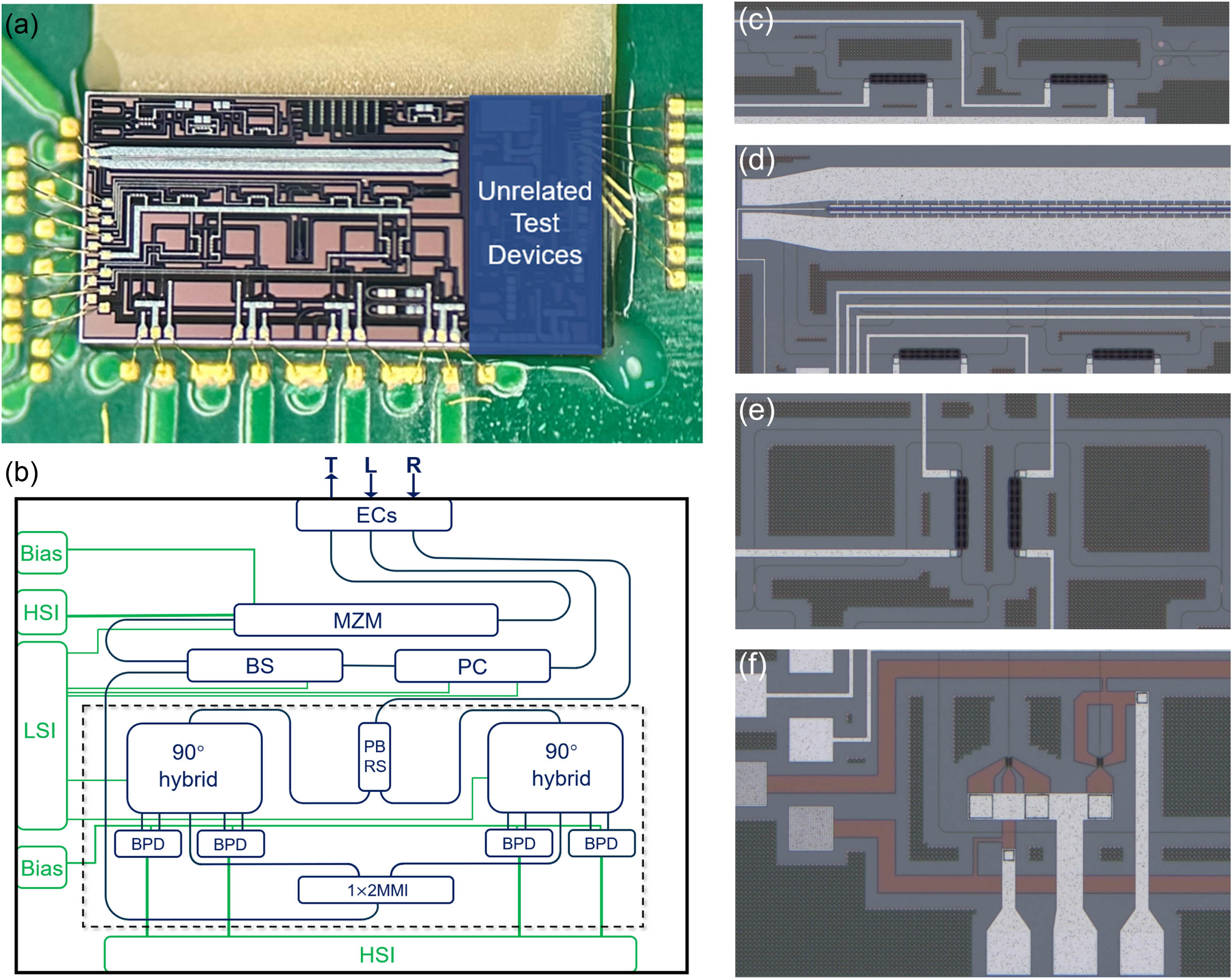
Fig. 1. (a) Microscope image of the photonic integrated circuit (PIC). (b) Schematic of the PIC. EC, edge coupler; PC, polarization controller; BS, beam splitter; MZM, Mach–Zehnder modulator; PBRS, polarization beam rotator splitter; MMI, multimode interferometer; BPD, balanced photodetector; LSI, low-speed electrical interface; HSI, high-speed electrical interface. “L”, “T”, and “R” denote the three edge couplers, serving as the input for the light source, the output for modulated laser pulses, and the input for RBS light, respectively. The arrangement of the elements and waveguides in the sketch is consistent with the chip in practice except for the electrical wires, while the aspect ratio is adjusted for a better view. (c)–(f) Magnified micrographs of the PC, MZM, 90° hybrid, and BPD.

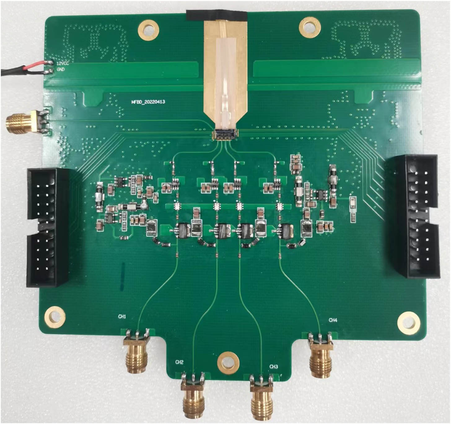
Fig. 2. Image of the packaged PIC for the DAS interrogator.

Fig. 3. Schematic of the DAS system based on TGD-OFDR. PIC, photonic integrated circuit; TIA, transimpedance amplifier; EDFA, erbium-doped fiber amplifier; PZT, piezoelectric transducer; SG, signal generator; LFM, linear frequency modulator; AWG, arbitrary waveform generator; DAQ, data acquisition card; DSP, digital signal processing.

Fig. 4. Experiment setup and results for tests on the receiver. (a) Schematic diagram of the test system. (b) Spectrum of VTE with 80 MHz frequency shift. (c) Spectrum of VTM with 80 MHz frequency shift. (d) Sideband suppression ratio (SSR) of VTE (blue) and VTM (red) over 2 h. Values at the starting time correspond to results in (b) and (c), respectively.

Fig. 5. Demodulation results for the 12.1 km sensing fiber. (a) Normalized intensity traces with polarization fading suppressed (green) and with fading (red and blue). (b) Distance–time distribution of the differential phases along the fiber, with a vibration applied at around 12.1 km. (c) Phase standard deviation (SD) trace along the fiber with a spatial resolution (SR) of 1.14 m. (d) Waveform of the 100 Hz vibration from 10 ms to 40 ms. (e) Power spectral density (PSD) of the measured variation. The self-noise level is shown as the red dashed line.

Fig. 6. Demodulation results for the 49.0 km sensing fiber. (a) Normalized intensity traces with polarization fading suppressed (green) and with fading (red and blue). (b) Distance–time distribution of the differential phases along the fiber, with a vibration applied at around 49.0 km. (c) Phase SD trace along the fiber with 3.78 m SR. (d) Waveform of the 100 Hz vibration from 40 ms to 70 ms. (e) PSD of the measured variation.

Fig. 7. Demodulation results for the 74.1 km sensing fiber. (a) Strain resolution distribution along the sensing fiber. (b) Waveform of the 100 Hz vibration from 10 ms to 50 ms.