Line-field Confocal Optical Coherence Tomography (LC-OCT) is a recently introduced optical imaging technique combining the principles of time-domain OCT and reflectance confocal microscopy (RCM) with line illumination and line detection using broadband near infrared light. LC-OCT performs two dimensional (2D) and three-dimensional (3D) imaging with a quasi-isotropic resolution of ∼1 μm [1–4]. Up to now, LC-OCT has been applied to skin imaging for healthy skin characterization [5, 6] and early detection and diagnosis of various skin diseases including skin cancers [7–10]. LC-OCT provides images with cellular resolution similar to histology, while being non-invasive.

As in OCT and RCM, the contrast of LC-OCT images originates from the backscattering of light, due to refractive index inhomogeneities within the sample. The amount of detected backscattered light is determined by three main optical parameters specific to the imaged sample [11]: the absorption coefficient μ_a, the scattering coefficient μ_s, and the scattering anisotropy factor g. μ_s and μ_a correspond to the probability per unit of distance of absorption or scattering events respectively and thus reflect the amount of absorbed and scattered light. g is defined as the average of the scattering angles cosines along the photon path and hence characterizes the directivity of the scattered light. These optical parameters rule the decay of the OCT image intensity with depth I(z), commonly described by a Beer-Lambert law in the single-scattering regime [12]:(1)Iz∝exp-2μzwhere μ = μ_a + μ_s is the attenuation coefficient, characterizing the attenuation of the incident light during in-depth propagation, due to absorption and scattering. The factor 2 accounts for round-trip propagation of light in the sample.

Beyond morphological information, LC-OCT images contain information on optical properties of the sample. Those optical properties are determined by the size, shape and density of tissue light scatterers (nucleus, mitochondria, cytoskeleton, extracellular fiber such as collagen) at cellular and sub-cellular levels. The extraction of optical properties would thus allow access to quantitative information complementary to the morphological information provided by the LC-OCT images. Optical properties could be used as a tool for tissue characterization and quantification of tissue structural changes, which could for instance occur during the development of a pathology.

Quantification of the attenuation coefficient μ using conventional OCT has been used for several biomedical applications, such as atherosclerosis plaque characterization [13], human brain cancer infiltration detection [14], glaucoma diagnosis [15], urothelial carcinoma staging and grading [16] or basal cell carcinoma characterization and subtypes differentiation [17]. Several methods have been developed to measure the attenuation coefficient μ, as reviewed by [12, 18]. The most common approach is to fit an exponential decay curve on the OCT image intensity as a function of depth to extract the attenuation coefficient μ. More recently, Vermeer et al. [19] introduced a new method for depth-resolved measurement of the attenuation coefficient. Based on two assumptions (the incident light is completely attenuated within the OCT imaging depth range and the backscattered light is a fixed fraction of the attenuated light), their approach provides a pixel-by-pixel estimation of μ, thereby producing attenuation maps with the spatial resolution of the OCT image.

In contrast, fewer work has been reported on the separate measurement of the optical parameters μ_a, μ_s and g using OCT. However, the interest in measuring the optical properties, and especially the scattering parameters μ_s and g, is that each of them provides different and complementary information on tissue structure. μ_s is determined by several factors, including the density, size and shape of the scattering particles, while g is defined by the size and shape of these particles [20]. The measurement of both parameters μ_s and g could therefore provide a comprehensive insight into tissue structural changes occurring in pathologies. The depth-resolved method is limited to the measurement of the attenuation coefficient μ due to its assumption that the backscattered light is a fixed fraction of the attenuated light.

A few methods based on curve-fitting allow the measurement of the optical properties μ_a, μ_s and g. Thrane et al. [21] introduced a model to extract the optical parameters μ_a, μ_s and g from the OCT image intensity with depth I(z). This approach consists in fitting a theoretical model on I(z), based on the extended Huygens–Fresnel (EHF) principle. This model was later applied to the skin to distinguish between biopsies of melanoma and benign nevi [22]. In this study, the different layers of skin have not been dissociated and the skin was considered as a monolayered tissue. Studies have been carried out to show the applicability to bilayered samples, however the model becomes cumbersome to implement [23]. Another simpler approach for extracting the optical properties from OCT images was introduced by Jacques et al. [24]. The authors proposed to extract the scattering properties μ_s and g from OCT images using a linear fit. The model, based on Monte-Carlo simulations, was designed for OCT in focus-tracking mode and RCM. It was validated on phantoms with known optical properties [25] and later applied to the extraction of scattering properties of various biological tissues including the skin [26, 27]. This model was also applied on bilayered tissues [28].

As a combination of RCM and OCT (in focus-tracking mode as will be described later), LC-OCT is particularly suitable for the application of the model developed by Jacques et al. [24]. Based on this model, we present a method to determine both μ_s and g from LC-OCT images of tissue-mimicking phantoms. Our approach provides the mean values of μ_s and g over a lateral field of view of 1.2 mm × 0.5 mm (x × y). It can be applied to monolayered and bilayered samples, where it allows extraction of μ_s and g of each layer. The method was experimentally validated against integrating spheres and collimated transmission measurements on a set of nine monolayered phantoms and two bilayered with distinct optical properties in terms of both scattering properties μ_s and g. The phantoms were made of a polydimethylsiloxane (PDMS) polymer including different types of scattering particles and aim at mimicking tissue scattering properties in the near infrared range. The developed method is simple to implement since it relies on a linear fit and a calibration using one of the fabricated phantoms whose scattering properties were determined by integrating spheres and collimated transmission. The method provides additional quantitative bulk information (i.e., at a macroscopic scale), complementary to LC-OCT images providing information at a microscopic scale.

In order to mimic optical properties of biological tissues such as skin [29–31], phantoms were designed with a scattering coefficient μ_s ranging from ∼2 to 20 mm⁻¹ and an anisotropy factor g from ∼0.6 to 1. Since most biological tissues have negligible absorption compared to scattering (scattering is 10–100 times higher than absorption in the near infrared spectrum [29]), we chose μ_a ≪ μ_s. In the following, we focus on the measurement of the scattering properties μ_s and g, neglecting the role of μ_a.

The phantoms are composed of a PDMS matrix (Sylgard 184 silicone Elastomer Kit, Neyco, France) with a refractive index of 1.42 at the wavelength of 800 nm [32, 33]. To create phantoms with various optical scattering properties, different micro- and nano-powders were added into the PDMS matrix: titanium dioxide (TiO₂) powder (Sigma-Aldrich Corporation, USA), zinc oxide (ZnO) powder (US Research Nanomaterials, Inc., USA) and silicon dioxide (SiO₂) powder (US Research Nanomaterials, Inc., USA). All powders have negligible absorption compared to scattering in the near infrared.

In order to select the appropriate scatterers to mimic optical properties of the skin, Mie theory (assuming spherical particles) was used to simulate μ_s and g values of the phantoms as a function of the refractive index, size and density of the particles embedded in PDMS. However, all the parameters necessary to predict the optical properties by Mie theory were not precisely known. For example, only the mean particle size was sometimes given by the manufacturer, without information on the size distribution. The refractive index of the nanoparticles was not provided either. For ZnO and SiO₂ particles, we approximated the refractive index by optical index values extracted from the literature at the 800 nm wavelength [34, 35]. For TiO₂ particles, a wide range of refractive indices was found [34, 36, 37], so an average of the different refractive indices reported in the literature was chosen. Ten different phantoms were fabricated. The detailed description of the composition of the phantoms is given in Table 1, with target values of μ_s and g computed using Mie theory when possible. The target values of μ_s and g are not given for phantoms 0 and 3 due to the lack of precise information on the size of the particles used (<5 μm).

The PDMS matrix was fabricated using a ratio of 10:1 by weight of PDMS pre-polymer and curing agent. All phantoms were prepared by first mixing the curing agent with a variable amount of scattering powder. The mixture was placed in an ultrasonic bath for 30 min to prevent particles aggregation, and then mixed with the PDMS pre-polymer. The obtained mixture was poured on a 40-mm diameter petri dish. The volume poured was chosen in order to obtain 1–2.5 mm thick phantoms, a thickness allowing their characterization by integrating spheres. Air bubbles were removed using a vacuum pump for 1 h, and the phantom mixture was finally cured for1 1/2 h at 80 °C.

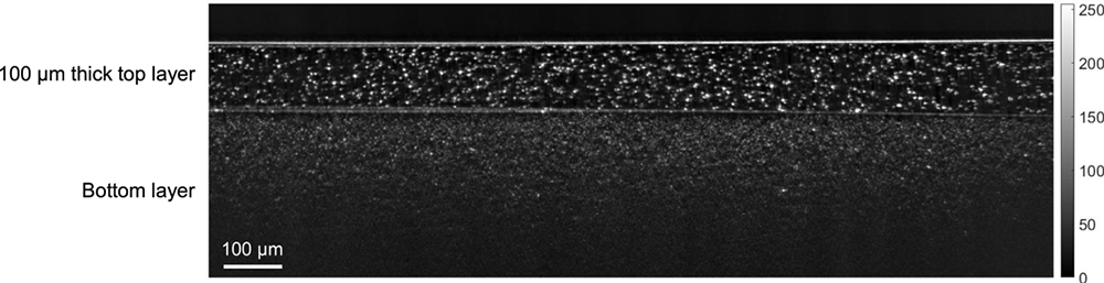
We also designed two bilayered phantoms with distinct optical properties in each layer, as listed in Table 2. To create the top layer, a small volume of the PDMS/scattering powder mixture was poured in a petri dish. The phantom was left for 24 h in a vacuum chamber at room temperature, allowing the mixture to spread into a thin layer before curing. This process allows to achieve a thickness of∼100 μm. Since this phantom is very fragile, another thicker phantom was fabricated using the same batch mixture, facilitating the measurement of the top layer scattering properties using integrating spheres and collimated transmission set-up. Once cured, the obtained top layer was stacked on a thicker phantom with different optical properties to create a bilayered phantom, using a small drop of paraffin oil (refractive index of∼1.47) between the two layers for optical contact. A representative LC-OCT image corresponding to a vertical image (i.e., cross-sectional view) of one of the bilayered phantoms is shown in Figure 1.

Mie theory allows to define target values for μ_s and g. However, as previously mentioned, the characterization of the optical properties by Mie theory is not very reliable due to uncertainties on the size distribution and the refractive indices of the particles used in our phantoms. Therefore, these target values are indicative values but cannot be used as reference values to compare with values obtained from LC-OCT images. Thus, the optical properties of our samples were characterized experimentally, using integrating spheres and collimated transmission devices.

Integrating spheres measurement is a common method to measure optical properties of samples [38–40]. It consists in measuring the diffuse reflectance and diffuse transmittance of a sample using a set-up with one or two hollow spheres with a diffuse reflective internal coating. The absorption coefficient μ_a and the reduced scattering coefficientμs'= μs(1-g) are then derived from these two measurements using theoretical models [41]. In order to separate the reduced scattering coefficientμs' into the scattering coefficient μ_s and the scattering anisotropy factor g, a collimated transmission measurement is required. This measurement is obtained by collecting the ballistic light from a laser beam propagating perpendicularly to the phantom. A more detailed description of integrating spheres and collimated transmission measurements can be found in [42].

We used a set-up with two integrating spheres (2″ Integrating Sphere IS200-4, Thorlabs, USA). The sample was placed between the two spheres. Light from a high-power broadband Xenon light source (HPX 2000, Ocean Insight, Dunedin, Florida) was guided to one of the two spheres using a 50/125 optical fiber and collimated into a 6-mm diameter beam. Diffuse reflected and transmitted light were collected using an optical fiber (plastic fiber, PMMA Toray, 50-cm long, 1-mm diameter, 0.22 NA) coupled to a spectrometer (AvaSpec2048, Avantes, Netherlands). Collimated transmission measurement was carried out with a monochromatic fiber laser diode at 785 nm (Micron Cheetah, Sacher LaserTechnik, Germany). The laser beam was collimated at the fiber output and its diameter was reduced using a diaphragm. The phantom was placed a few cm behind the diaphragm, perpendicular to the laser beam. A collection fiber (105 μm core diameter, 0.1 NA), connected to the spectrometer, was placed one meter behind the phantom in order to collect the ballistic light. Due to its small diameter, low numerical aperture and large distance to the sample, the fiber acts as a pinhole rejecting scattered photons.

All measurements were corrected for dark noise and normalized with respect to blank measurements without sample. The optical properties were computed using the Inverse Adding-Doubling (IAD) algorithm developed by Prahl [43]. μ_s and g were determined at the wavelength of 785 nm. Despite the slight difference in wavelength from that of the LC-OCT device centered at 800 nm, the difference in μ_s and g values between these two wavelengths can be considered negligible compared to the accuracy of our measurements [39], allowing for comparison of integrating spheres and collimated transmission measurements with measurements obtained from LC-OCT images.

In practice, the collimated transmission measurement could not be performed on some of the highly concentrated phantoms (3, 5, 7 and 9) since the ballistic intensity was too weak. However, phantoms 3, 5, 7 and 9 are made of the same scattering particles as phantoms 1, 4, 6 and 8 respectively. Since g is ruled by particle size and shape [20], the values of g of phantoms 3, 5, 7 and 9 were considered identical to those of phantoms 1, 4, 6 and 8 respectively.

For bilayered phantoms, the top and bottom layers were analyzed separately since integrating spheres and collimated transmission do not allow to separate the scattering properties of two stacked layers. As previously mentioned, since the 100 μm-thick top layer was very fragile, the scattering properties of the top layer were measured on a thicker phantom fabricated with the same batch mixture as the thin top layer.

The LC-OCT device used in this work is described in [1–4]. The device is based on a Linnik interferometer with a 0.5 NA water-immersion microscope objective in each arm. A supercontinuum light source centered around 800 nm is used to generate spatially coherent ultra-broadband light. Line illumination of the sample is achieved using a cylindrical lens, and backscattered light is detected with a line camera. LC-OCT is capable of generating 2D vertical section images (i.e., cross-sectional views, x × z) and horizontal section images (i.e., en-face views, x × y). By combining the depth and lateral scans used to generate 2D images, 3D images can also be obtained, with a quasi-isotropic resolution of∼1 μm over a field of view of 1.2 mm × 0.5 mm × 0.5 mm (x × y × z). During imaging, samples are placed in contact with a glass plate to stabilize them and maintain them at the position corresponding to the working distance of the microscope objective. Paraffin oil is placed between the phantoms and the glass plate to minimize parasitic reflections at the interface.

Within the single-scattering regime and in focus-tracking mode, the reflectance R(z) measured along an A-scan acquired by OCT or LC-OCT image (i.e., the depth-dependent fraction of incident light backscattered and collected by the device) can be described by an exponential decay with depth [29]:(2)Rz=ρexp-2μz.ρ is the fraction of light backscattered at the focus into the collection solid angle of the LC-OCT microscope objective; μ = μ_s + μ_a is the attenuation coefficient previously introduced, and the factor 2 accounts for round-trip attenuation inside the sample. Since the factor1μs represents the average distance between two scattering events [44], the single scattering regime is valid as long as μ_sz ≤ 1. This model of the LC-OCT signal is therefore valid for media with low scattering properties or/and at shallow penetration depths.In order to be able to measure the optical properties of more scattering media, Jacques et al. [29] proposed a model, also based on an exponential decay law, allowing to take into account forward directed multiple scattering:(3)Rz=ρexp -2μeffz,where(4)μeff=Gg,NA(μa+a(g)μs)ρ =μs∆zbg, NA,where G(NA,g), a(g) and b(g,NA) are model parameters described in [24] and Δz the axial resolution of the imaging device. Note that in the case of RCM, the authors mention that a corrective factor may be necessary to account for a difference between the theoretical axial resolution of the RCM system and the effective axial resolution to be taken into account in the model [28]. In the case of LC-OCT, the axial resolution was computed as∆Z=2 log (2)πλ2Δλ=1.2 μm and no corrective factor was required based on results presented later in this paper.

G(NA,g) describes the average optical path length traveled by the photons collected by the OCT system, taking into account the numerical aperture NA and the scattering anisotropy factor g of the imaged sample. This term takes into account the fact that photons emitted at the edge of the beam travel a longer optical path than photons emitted on the optical axis. For NA = 0.5 (numerical aperture of the LC-OCT device), G is close to 1 [24].

a(g) is called the scattering efficiency factor. It reflects the contribution of forward scattered photons, i.e., serpentile photons. Serpentile photons can contribute to the backscattered intensity because of their trajectory similar to that of ballistic photons. Then, if they follow a serpentile trajectory on the return path, photons can contribute to the collected intensity. Thus, serpentile photons slow down the extinction of the incident intensity by scattering in the sample. This effect has been formalized in the form of a function a(g):(5)ag≈u1-e-(1-g)v/wwith u, v, and w parameters determined by Monte-Carlo simulations [24, 26]. For small values of g (isotropic scattering medium), a(g) is close to 1, which implies that μ_eff = μ as in the single-scattering regime. However, for values of g tending towards 1 (highly forward scattering medium), a(g) tends towards 0, leading μ_eff < μ, meaning that attenuation of light is slowed down by the contribution of serpentile photons. The authors have shown that this modeling of the contribution of multiple forward scattered photons is valid as long as μ_sz ≤ 3 [25]. However, this modeling does not take into account the possible contribution of photons multiply scattered along a non-ballistic optical path. This typically allows the measurement of scattering coefficients on the order of 10 mm⁻¹ down to a depth of 400 μm, and down to 200 μm for the most scattering phantoms (up to 20 mm⁻¹). Jacques’ model thus appears to be very well adapted to the measurement of optical properties of biological tissues imaged with LC-OCT.

b(g,NA) is qualified as collection efficiency and represents the fraction of light scattered from probed volume and collected by the microscope objective of the LC-OCT device. b(g,NA) is ruled by the phase function of the sample, described by the Henyey–Greenstein function in this model [45], and the collection angle of the microscope objective, given by the value of NA.

In this modeling of R(z), ρ and μ_eff can be considered as experimental observables and can be extracted from an LC-OCT image as described in the following section.

The principle of our method consists in measuring μ_eff and ρ parameters from an LC-OCT image, and to convert these parameters into the optical properties μ_s and g using the previously described model proposed by Jacques et al. To do so, a 3D LC-OCT image is acquired for each phantom. The 3D image results from the acquisition of a stack of 2D LC-OCT horizontal images (i.e., en-face sections). Each image of the stack is obtained by demodulating the interferometric lines acquired successively in the horizontal plane during the lateral scan, using a phase-shifting algorithm [4]. No processing is applied to the LC-OCT images in order not to distort the measurement of the scattering properties. The first step is to compute the reflectance R(z). Since phantoms have a homogeneous distribution of scattering particles, the mean reflectance R(z) in the 3D image is considered. All A-scans within the 3D LC-OCT image are averaged to obtain a mean depth-dependent intensity I(z). Since the phantoms are composed of discrete scattering particles, averaging all A-scans within the 3D image provides the smoothest possible intensity profile I(z), which will then help maximize the quality of the linear regression that will be applied as described in the following. The mean reflectance R(z) is then obtained by converting I(z) into dimensionless units of reflectance using a calibration constant f: R(z) = fI(z). This simple calibration using a proportionality factor is made possible since LC-OCT operates in focus-tracking mode and thus does not require confocal functions to be taken into account as is sometimes the case with conventional OCT [12, 18].

ρ and μ_eff are extracted by applying a least square linear regression on log R(z) (Fig. 2), from the surface of the sample down to a depth of about 150 μm. ρ is obtained from log ρ, which corresponds to the intercept with depth z = 0 representing the interface between the glass plate and the phantom (intensity peak visible at z = 0 in Fig. 2); μ_eff is given by half the slope of the linear regression.

Finally, the resulting parameters ρ and μ_eff extracted from the 3D LC-OCT image are mapped to the optical properties μ_s and g using the model by Jacques et al. previously described. Several ways can be considered to recover μ_s and g from μ_eff and ρ using equations (4) of the Jacques’ model. In this paper, the following relationship was used considering μ_a ≪ μ_s:(6)μeffρ=aGbΔz.The expression ofμe f fρ, proposed by Jacques et al. in [24], is a function of λ, NA and g and is independent from μ_s. The curveμe f fρ as a function of g (for λ = 800 nm and NA = 0.5), shown in Figure 3, can thus be used to compute the value of g from the two observables ρ and μ_eff. μ_s can then be recovered from the value of μ_eff and g using equations (4). The resulting μ_s and g values correspond to the mean optical properties over the LC-OCT lateral field of view of 1.2 mm × 0.5 mm (x × y).

For bilayered phantoms, two distinct areas of linear decay can be observed on the averaged intensity profile plotted in Figure 4, corresponding to the two layers of the sample. Since the two layers have different optical properties, they exhibit different slopes. As for the monolayered phantoms, the intensity peak at depth z = 0 indicates the interface between the glass slide and the phantom. In this example, the intensity peak around 110 μm depth shows the interface between the two layers. To extract the values of μ_eff and ρ in each layer (noted ρ_top, μ_efftop and ρ_bottom, μ_effbottom), the two layers are segmented by manually delineating the two areas of linear decay. A linear fit is then applied separately on each layer, as depicted in Figure 4. In the bottom layer, the intercept with the interface between the two layers (at depth z = 110 μm) corresponds to log(ρbottome-2μefftopδz) due to attenuation in the top layer of thickness δz. ρ_bottom is retrieved fromρbottome-2μefftopδz by multiplying it with a correction factorC=e2μefftopδz to compensate from attenuation in the top layer.

The resulting parameters ρ_top, μ_efftop and ρ_bottom, μ_effbottom are then mapped to the optical properties μ_s and g in each layer using the model by Jacques et al. as described in the previous section.

As introduced in the previous section, the mean intensity I(z) (in gray levels) in an LC-OCT image can be converted into dimensionless units of reflectance R(z) using a calibration constant f such that R(z) = fI(z). To determine f, one of the phantoms was used as a calibration phantom. On the one hand, μ_s and g of the calibration phantom were obtained from integrating spheres and collimated transmission measurements. Using the model of Jacques et al. [24], the ratiorcalib=μeffcalibρcalib was determined from the g value measured for this phantom. On the other hand, a 3D image of the calibration phantom was acquired. The values of I₀ρ_calib and μ_calib were extracted by applying a linear regression on the mean intensity I(z) in the image. Knowing the value of the expected r_calib ratio, the value of ρ_calib can be obtained from μ_effcalib. A calibration factor f can then be calculated as the ratio of the expected value for ρ_calib and the value of I₀ρ_calib measured from the 3D LC-OCT image:(7)f=ρcalibI0ρcalib.Other calibration approaches can be considered, but this approach has the advantage that it does not involve the value of μ_s measured using integrating spheres and collimated transmission. This is an interesting feature: while the value of g is independent from particle density, this is not the case of μ_s. Since integrating spheres and collimated transmission measurements are performed on a field of 6 mm diameter and LC-OCT measurements on a field of the order of 1 mm, it is preferable in case of particle density heterogeneities in the calibration phantom to use only the g value obtained using integrating spheres and collimated transmission to calibrate reflectance in LC-OCT images.

For each phantom, integrating spheres and collimated transmission measurements were performed three times. Mean values of μ_s and g obtained with integrating spheres and collimated transmission were calculated from these three measurements.

Since LC-OCT measurements are based on a calibration performed with a calibration phantom whose optical properties are obtained by integrating spheres and collimated transmission measurements, the uncertainties of the integrating spheres and collimated transmission method have a significant impact on the accuracy of LC-OCT measurements of μ_s and g. Values of μ_s and g were computed from mean values of μ_s and g obtained from three 3D LC-OCT image, and uncertainties on LC-OCT measurements were estimated as follows: first, the uncertainty on the calibration factor f was estimated from uncertainties obtained on μ_s and g values of the calibration phantom measured using integrating spheres and collimated transmission measurements. From the resulting uncertainty on f, the uncertainty on ρ, due to calibration, was obtained for each fabricated phantom. Additional uncertainties on ρ and μ_eff were experimentally observed due both to least square linear regression on the intensity depth profile extracted from the 3D image and to slight variations of ρ and μ_eff from one image to another of the same phantom. Finally, uncertainties on μ_s and g were evaluated for each fabricated phantom by propagating total uncertainties on ρ and μ_eff through the model of Jacques [24] previously described.

Comparisons of μ_s and g values of monolayered phantoms obtained from LC-OCT mean intensity depth profiles and integrating spheres and collimated transmission measurements are given in Figures 5 and 6. Additionally, values of μ_a obtained from integrating spheres and collimated transmission measurements are given in Figure A1 of Appendix A.

First of all, one can observe that the optical scattering properties obtained correspond to the range of properties targeted, with μ_s values between 1 and 25 mm⁻¹ and g values between 0.68 and 0.94. The obtained results confirm that μ_a ≪ μ_s for all phantoms. For phantoms made of the same particles (in terms of refractive index and size), one can notice that the value of μ_s increases with the particle concentration, in agreement with Mie theory. The measured values of μ_s do not correspond exactly to the theoretical values, but the order of magnitude is similar. As stated earlier, the theoretical values are indicative due to uncertainties in the size and refractive index of the scattering particles. Moreover, it should be noted that during the fabrication process, particle losses may have occurred when pouring the particle/hardener mixture into the prepolymer, which may also contribute to some deviations in μ_s. Concerning the g parameter, we can note that here again the values of g for the phantoms 1, 4 and 8 have the same order of magnitude compared to Mie theory. However, the value of g obtained for phantom 6, composed of 400 nm SiO₂ particles, is largely higher (0.94) than the target value (0.7) and is equivalent to the value of g obtained for phantom 8, composed of SiO₂ particles of larger size (1 μm). A possible explanation could be the aggregation of 400 nm particles into larger particles, of the order of 1 μm.

When looking at the comparison of μ_s and g values between the two measurement methods, results show that, for phantoms 1–6 and 8, LC-OCT is capable of providing measurements of optical properties consistent with those obtained by integrating spheres and collimated transmission measurements, with overlapping error bars (nearly overlapping for the μ_s measurement for phantom 2). For phantoms 7 and 9, one observes a good agreement of g values between the two methods. On the other hand, we observe a significant discrepancy between the value of μ_s measured by integrating spheres and collimated transmission and that measured by LC-OCT. To date, we have no definitive explanation for this discrepancy, but a potential explanation could be the presence of aggregates in phantoms. As shown by high-resolution bright field microscopy images (acquired with a 1.35 NA objective) given in Figure 7, aggregates could be observed in some areas of our phantoms, while other areas were well homogeneous. We also observed a greater number of aggregates as we penetrated deeper into the phantoms. LC-OCT images covered a 1.2 mm × 0.5 mm × 0.5 mm (x × y × z) field of view, and were acquired in regions excluding aggregates (or at least minimizing their number). In contrast, the integrating spheres and collimated transmission measurements are based on transmission through the entire thickness of the phantom and over a lateral diameter of 6 mm, which potentially takes into account much more aggregates than LC-OCT. This issue shows the limitation of our fabrication process. In the future, it would be necessary to revise the manufacturing process, for instance with better mechanical mixing to improve homogeneity.

The measurements of μ_s and g have fairly high uncertainties, represented by the error bars in Figures 5 and 6. The error bars associated with the integrating spheres and collimated transmission measurements reflect the difficulty to perform these measurements. Indeed, although being a reference method, the collimated transmission measurement is an experimental measurement that was difficult to perform in a repeatable way and that required improvements to the initial setup. In particular, since the phantoms were not perfectly flat, the ballistic beam could be deflected. It was therefore necessary to readjust the injection in the collecting fiber for each phantom. Another potential source of error in the collimated transmission measurement is the contribution of multiple scattered photons to the ballistic intensity when the value of g is high. The proportion of scattered photons collected compared to ballistic photons depends on the scattering properties and on the acceptance angle of the collection system. In this paper, the contribution of multiple scattering to collimated transmission was minimized at best using a fiber with a small core, low numerical aperture and placed far from the sample allowing to minimize the collection angle. Experimental difficulties lead to uncertainties not only on μ_s and g values determined with integrating spheres and collimated transmission, but also on LC-OCT measurements since the calibration is performed using a phantom with optical properties determined by this method, as explained in Section 2.4. When propagated through the model, these errors are amplified for high values of μ_s and g. This is why the error bars are strongly dependent on the optical properties of the phantoms. Thus, they are the widest for phantoms 6–9 which have a high value of g.

In summary, despite the issues encountered with phantoms 7 and 9, results obtained show that our measurement method is well suited to samples with medium to high scattering anisotropy (0.7 < g < 0.9) and scattering coefficients μ_s up to 12 mm⁻¹, which already allows for application to biological tissues.

The results obtained on the bilayered phantoms are shown in Figure 8. The two layers of the bilayered phantoms have very different values of μ_s and g. The results show that for each layer, LC-OCT provides optical properties that are consistent with those obtained by the integrating spheres and collimated transmission method, with overlapping error bars. A very good agreement of g values can be observed between the two measurement methods, both for the top and bottom layers of the two bilayer phantoms.

Concerning μ_s values, one can also observe a good agreement for all layers. Overall, the difference between the two measurement methods on μ_s remains of the same order as the difference obtained on the monolayered phantoms. One can notice that the value of μ_s in the bottom layer of the bilayer phantom 2 is slightly lower than the value of μ_s obtained with the monolayer phantom 5 alone, a difference that can possibly be explained by a more important contribution of multiple scattering than with the monolayer phantom 5 since the linear regression on the bottom layer is applied deeper (from 100 to 200 μm). The model of Jacques et al. takes into account the multiple scattering in certain extent and when scattering is directed forward. In order to better account for multiple scattering in its entirety, multiple scattering models such as the EHF model proposed by Thrane et al. [21] could be used. However, the investigations of the EHF model carried out so far have not been conclusive and have led to unrealistic values of optical properties, an issue that was previously mentioned in [46]. It was suggested in [18] that the model needs a priori knowledge of μ_s or g since they are co-dependent parameters in the model. Moreover, this model is not yet suitable for the application to multilayered samples due to its complexity.

Nevertheless, our results obtained on bilayered phantoms demonstrate the potential of LC-OCT to provide layer-based measurements of distinct μ_s and g values from a single 3D image, unlike the integrating spheres and collimated transmission method which requires the two layers to be analyzed separately. Compared to the current state of the art, the application of our method on bilayered phantoms with different values of μ_s and g in each layer is innovative since previously reported multilayered phantoms have identical g values in all layers. However, our fabrication process would need to be improved for obtaining a more homogeneous thin top layer. Indeed, as for monolayered phantoms, aggregate deposition in the bottom of the thin layers has sometimes been observed. One solution could be to cut a thin layer from a thicker sample that would be more homogeneous.

We have developed a method for measuring the scattering coefficient μ_s and the scattering anisotropy factor g of a sample from a single 3D image of that sample acquired by LC-OCT. Our approach is based on the extraction of two observables ρ and μ_eff from the LC-OCT image, by applying a linear fit to the mean intensity depth-profile within the 3D image (in logarithmic scale). Using a calibration with a phantom of known optical properties and a model previously introduced in the literature [24], the values of ρ and μ_eff can be mapped to the values of the scattering parameters μ_s and g. We tested our method on PDMS phantoms containing nano- and micro-scattering particles mimicking optical properties of typical biological tissues, and compared it to another commonly used method based on integrating spheres and collimated transmission measurements. The values obtained measured by LC-OCT are consistent with those obtained from the integrating spheres and collimated transmission measurements, suggesting that LC-OCT is a relevant tool to measure the optical scattering properties of semi-transparent samples.

Compared to integrating spheres and collimated transmission measurements that require manipulating the sample (place it between the spheres, then move it on the collimated transmission bench) and involves constraints on the sample physical characteristics (minimum size corresponding to the beam diameter, minimum thickness to be placed between the two spheres without risk of damaging the sample, maximum thickness for the collimated transmission to be possible), LC-OCT does not require specific sample handling and constraints, which simplifies the measurement procedure and would facilitate in vivo measurements of μ_s and g. Moreover, LC-OCT allows measurements on multilayered samples with distinct optical properties in each layer, using a single 3D image, unlike integrating spheres and collimated transmission which require analyzing the different layers separately. In this paper, we demonstrate the applicability of our method to bilayered samples, with the ultimate aim of applying the approach to the two main layers of the skin, the epidermis and the dermis. However, our method is not limited to two layers, but could be applied to multilayered samples (>2) following the same approach as for bilayered samples, as described in Section 2.3.4.

Our layer-based approach is interesting since few papers have reported measurement by OCT of 1 distinct μ_s and g values on multilayered samples [47, 48]. Compared to these previous works, our developed method has the advantage of being very simple to implement since it is based on a linear fit and a scattering model, and requires only a preliminary calibration step, using a phantom with known optical properties. Since LC-OCT is based on time-domain OCT with dynamic focusing, LC-OCT measurements do not require corrections accounting for the confocal function of the focusing lens [12]; this is another reason why LC-OCT is particularly appropriate for the application of Jacques’ model.

The model of Jacques et al. takes into account multiple scattering when scattering is strongly directed forward, but it does not extensively account for multiple scattering as the extended Huygens–Fresnel (EHF) model does [21]. However, investigations of the EHF model have not yet given conclusive results on our phantoms. Moreover, Jacques’ model does not account for absorption, which restricts application to purely scattering samples (excluding for instance biological tissues with a high concentration of blood vessels or melanin). Our approach is also limited by the calibration step using a phantom with optical properties determined by integrating spheres and collimated transmission measurements. In particular, the collimated transmission measurement is complex to implement, leading to significant uncertainties of the measurement of μ_s and g, especially for high values of μ_s and g. Other techniques for measuring g (e.g., goniometry) could be investigated to reduce the uncertainties of collimated transmission measurements. However, goniometry, as collimated transmission, is complex to perform and requires constraints on the geometry of the samples in order to be able to collect scattered intensity from all angles [49].

Since LC-OCT provides morphological images, a future prospect could be to perform spatially resolved measurements of μ_s and g in a horizontal plane, in addition to the layer-based measurements obtained on the bilayered phantoms. Such spatially-resolved measurements could be obtained by dividing the 3D LC-OCT image into macro-voxels, in which values of μ_s and g could be extracted using the mean intensity depth profile in each macro-voxel. A macroscopic spatial distribution of μ_s and g could then be obtained. Further investigation is required to apply our method to biological tissues. LC-OCT is an imaging modality designed for biological tissue imaging, and in particular for skin imaging in vivo. Applied to biological tissue, the presented method could provide LC-OCT with the ability to quantify the scattering properties of tissue imaged in vivo, complementary to the qualitative information provided by the high-resolution of images. Potentially, the method could be used in vivo to characterize biological tissues and monitor structural changes that occur during the development of a pathology.