Generic nonlinear error compensation algorithm for phase measuring profilometry

Xin Yu; Shanshan Lai; Yuankun Liu; Wenjing Chen; Junpeng Xue; Qican Zhang

doi:10.3788/COL202119.101201

Abstract

In this Letter, the periodical errors, which are caused by the nonlinear effect of the commercial projector and camera, are analyzed as a more generic single-coefficient model. The probability density function of the wrapped phase distributions is used as a tool to find the compensation coefficient. When the compensation coefficient is detected, on the premise of ensuring accuracy, a correlation algorithm process is used to replace the traditional iterative process. Therefore, the proposed algorithm improves the efficiency of coefficient detection dramatically. Both computer simulation and experiment show the effectiveness of this method.

Keywords

nonlinear response phase error probability density function three-dimensional sensing

1. Introduction

Three-dimensional (3D) measurement technology^[1–3] is more and more closely related to our life. Among them, phase measuring profilometry (PMP) based on the phase-shifting method is widely used in biomedical research^[4], industrial design, quality detection, and other industries^[5] due to its advantages of high accuracy and high reliability. Usually, a series of sinusoidal fringe patterns are projected on the surface of the object, and then the camera captures the fringes modulated by the object height function. The phase distribution is obtained by analyzing the fringe patterns, and then the 3D information of the object can be restored by phase unwrapping^[6,7] and system calibration techniques. Since the 3D information of the object is calculated from the phase, the precision of phase calculation is very important to the measurement. However, the nonlinear response of the commercial projector–camera system often introduces the periodic phase error. It greatly influences the measurement accuracy.

Many researchers have developed many methods, which can be roughly divided into two categories. The first category is called preprocessing, that is, to change the fringes before projection in order to obtain the ideal phase distribution. One solution is called gamma correction^[8–13]. It is used to find the most proper gamma and encode it in the projected fringe patterns to produce the ideal sinusoidal fringes. Another method is called defocusing technology^[14–17], in which the ideal sinusoidal fringe is obtained by defocusing the binary fringe to reduce the effect of the nonlinear response. However, it is challenging to precisely control the defocusing degree.

The second category is called post-processing. It is to obtain the ideal phase distributions by compensating the nonlinear errors from the distortion fringe^[18–21]. Yatabe et al.^[18] proposed a general framework for approximating and compensating the nonlinear distortion of a fringe to estimate an inverse map of the nonlinearity from the observed images. Zhang et al.^[19] compensated for the phase errors by generating a look-up-table (LUT) between the phase error values and the corresponding phase values. Pan et al.^[20] used an iterative algorithm to reduce the phase errors owing to non-sinusoidal waveforms. Cai et al.^[21] employed the Hilbert transformation (HT), which produces a phase error model with the identical amplitude and opposite direction compared with the phase error model without HT.

Sign up for Chinese Optics Letters TOC. Get the latest issue of Chinese Optics Letters delivered right to you！Sign up now

To the best of our knowledge, when the nonlinear errors are periodical, the probability density function (PDF) of the wrapped phase can be used as a criterion to identify the nonlinear effect quantitatively. In Ref. [8], the PDF tool is used to find the systematical gamma to fulfill a pre-correction process. In our previous work^[22], we used this tool to launch a post-correction process, while it is difficult to adjust the systematical gamma. Two coefficients need to be detected, and an iteration process is needed for each set of candidates, which will increase the computational complexity dramatically. In this Letter, a new nonlinear error model, the single-coefficient model, is presented. It means that only one coefficient $K_{2}$ is adequate to fulfill the compensation. It can greatly simplify the searching process. Furthermore, the correlation process, which is to find the optimal coefficient from the pre-generated simulated PDF curves without any iteration process, can make the searching process even faster. The experiment shows that the proposed method is flexible, has high accuracy, and can lead to a fast, even a real-time, phase error compensation.

2. Principle

2.1. Phase error introduced by the nonlinearity

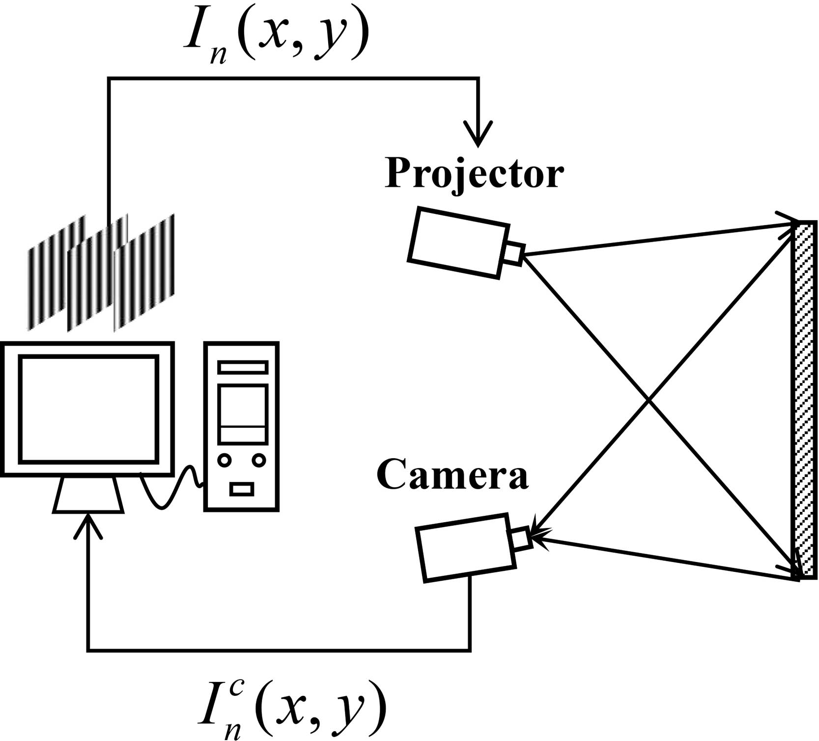
A digital fringe projection system is shown in Fig. 1. The digital projector is used to project the computer-generated fringe to the object surface. The CCD camera is used to capture the fringe patterns modulated by the height of the object.

Figure 1.Fringe projection system.

The computer generates ideal sinusoidal fringes. Its intensity can be expressed as $I_{n} (x, y) = a (x, y) + b (x, y) \cos [φ (x, y) + δ_{n}],$ (1)where $(x, y)$ denotes an arbitrary point in the pattern, $a (x, y)$ is the ambient light, $b (x, y)$ is the fringe modulation, $φ (x, y) = 2 π f x$ is the ideal unwrapped phase, and $δ_{n} = 2 π n / N$ is the phase shift of each of the $N$ fringe patterns, with $n$ from 0 to $N - 1$ .

Because of the intrinsic gamma effect of the commercial projector–camera system, as well as the reflectivity of the object surface and ambient light, in fact, the captured fringe is $I_{n}^{c} (x, y) = R (x, y) {[I_{n} (x, y)]}^{γ} + I_{0},$ (2)where $R (x, y)$ is the reflectivity of the objective, $I_{0}$ is the ambient light, and $γ$ represents the system gamma, which introduces the high-order harmonics into the fringes. The distorted fringe can be rewritten as the following form. For convenience, the $(x, y)$ will be omitted: $I_{n}^{c} = A + \sum_{i = 1}^{\infty} B_{i} \cos [i (φ + δ_{n})],$ (3)where $A = R a + I_{0}$ and $B_{i} = R b_{i}$ are the DC component and $i$ -order harmonic component, respectively. It is easy to know that the ideal wrapped phase can be calculated from the following form. Without special instructions, the phase below refers to the wrapped phase: $φ = - \arctan (\frac{\sum_{n = 0}^{N - 1} I_{n} \sin δ_{n}}{\sum_{n = 0}^{N - 1} I_{n} \cos δ_{n}}) .$ (4)

We only consider harmonics up to the fifth order when $N = 3$ . Because as the harmonic order gets higher, the amplitude gets smaller and can even be ignored. But, the following derivation can be extended to higher-order harmonics and other phase-shifting methods easily. Using Eqs. (3) and (4), the measured phase can be rewritten as $φ' = - \arctan {\frac{\sum_{n = 0}^{2} {A + \sum_{i = 1}^{5} B_{i} \cos [i (φ + δ_{n})]} \sin δ_{n}}{\sum_{n = 0}^{2} {A + \sum_{i = 1}^{5} B_{i} \cos [i (φ + δ_{n})]} \cos δ_{n}}} .$ (5)

The measured phase $φ'$ distorted by the nonlinearity can be considered as the sum of the ideal phase $φ$ and the phase error $Δ φ$ ^[20]. Thus, the phase error is $Δ φ = φ' - φ .$ (6)

From Eqs. (4), (5), and (6), the phase error can be derived as the following form: $Δ φ = - \arctan [\frac{(B_{2} - B_{4}) \sin (3 φ) + B_{5} \sin (6 φ)}{B_{1} + (B_{2} + B_{4}) \cos (3 φ) + B_{5} \cos (6 φ)}] .$ (7)

In order to eliminate the effect of the reflectivity $R$ , as well as $B_{1}$ is certain to be greater than zero, $B_{1}$ is used to normalize Eq. (7). An accurate phase error model can be expressed as $Δ φ = - \arctan [\frac{(K_{2} - K_{4}) \sin (3 φ) + K_{5} \sin (6 φ)}{1 + (K_{2} + K_{4}) \cos (3 φ) + K_{5} \cos (6 φ)}],$ (8)where $K_{i} = b_{i} / b_{1}$ is the phase error coefficient, and $i = 2$ , 4, 5. Since the coefficients $K_{4}$ and $K_{5}$ are so small that they can even be ignored, the phase error model can be improved as $Δ φ ≅ - \arctan [\frac{K_{2} \sin (3 φ)}{1 + K_{2} \cos (3 φ)}] .$ (9)

After Taylor series expansion, Eq. (10) can be expressed as $Δ φ ≅ \frac{- 12 K_{2} \sin (3 φ) - 12 K_{2}^{2} \sin (6 φ) - 4 K_{2}^{3} \sin (9 φ)}{12 - 18 K_{2}^{2} + (36 K_{2} - 3 K_{2}^{3}) \cos (3 φ) + 18 K_{2}^{2} \cos (6 φ) + 3 K_{2}^{3} \cos (9 φ)} .$ (10)

Obviously, the proposed nonlinear error model is much more accurate than the approximated model in Eq. (12), which is used in our previous work^[22]: $Δ φ = - c_{1} \sin (3 φ) - c_{2} \sin (6 φ) .$ (11)

2.2. PDF-based algorithm

Let $P {\cdot}$ indicate the probability. The PDF can be calculated as the following: $F (m) = P {2 π m / M - π \leq φ_{m} < 2 π (m + 1) / M - π},$ (12)where $M$ means the number of sampling points, and it could be any appropriate integer. $m = 0, 1, 2, \dots, M - 1$ . The selection criteria for $M$ will be described below. The effect of the nonlinear error, when $N = 3$ , is shown in Fig. 2.

Figure 2.Nonlinear effect for (a) the wrapped phase and (b) the PDF curves.

In the ideal case, the probabilities of the wrapped phase values are equal, i.e., the PDF value is even^[22]. When there is any nonlinear response in the measurement system, the PDF curves will be changed accordingly. Figure 2(a) shows the nonlinear effect on the number of pixels in the two regions with selected phase values. The red regions $D_{m 1}$ and $D_{m 2}$ represent the measured phase, i.e., the case with nonlinearity, and the blue regions $D_{i 1}$ and $D_{i 2}$ represent the ideal case. Apparently, near $φ = π / 3$ and $- π / 3$ , the nonlinear errors reduce the number of pixels, and, near $φ = 2 π / 3$ and $- 2 π / 3$ , the nonlinear errors increase the number of the pixels. This phenomenon is consistent with the PDF curves, which are shown in Fig. 2(b). In the case with nonlinearity, the PDF curve has the peak values at the position with $φ = - 2 π / 3$ and $2 π / 3$ and has the minimum values at the position with $φ = π / 3$ and $- π / 3$ . Therefore, the selection of the M should be able to highlight this characteristic to the greatest extent.

The PDF curves and partial phase sampling regions with four kinds of different $M$ values are shown in the Fig. 3. Apparently, from Fig. 3(a), the position where the phase error is equal to 0, $- 2 π / 3$ , and $2 π / 3$ is mostly affected by the value of $M$ . For example, in the cases of $M = 64$ and $M = 32$ , when the phase value zero is the boundary of the sampling regions, the peak value will become two identical values, and, when the phase values $- 2 π / 3$ and $2 π / 3$ are not in the middle of the sampling region, the position of the peak values will also be deviated. It is easily seen that when $M$ is a multiple of three, the PDF curve has a higher quality. To ensure accuracy, 63 is considered the most appropriate number of sampling points here, and $F (m)$ should be 0.0159.

Figure 3.In the cases of different values of M: (a) PDF curves and (b) partial phase sampling regions.

2.3. Searching process by correlation

The process of finding the best coefficient $K_{2}$ and realizing the phase error compensation is shown in Fig. 3. First, the ideal wrapped phase distributions are generated by a computer. Second, a series of distorted phase values, which are influenced by a set of $K_{2}$ values, respectively, will be generated again from Eq. (10). Then, a series of PDF curves with different $K_{2}$ could be produced. When the real PDF curve is calculated from the measured wrapped phase, the most similar one will be located by a correlation process, which can be expressed as $R_{p} = \frac{\sum F \cdot F_{p}}{\sum F^{2} \cdot \sum F_{p}^{2}},$ (13)where $F$ means the real PDF curves, and $F_{p}$ means the $p$ th simulated PDF curve. In fact, Eq. (13) is the function to evaluate the similarity between the real PDF curve and simulated curves, and the PDF curve, which produces the maximum correlation value, is the right PDF curve. Then, the coefficient $K_{2}$ , which is 0.24 in Fig. 4, can be obtained.

Figure 4.Process of finding K₂ and compensation.

3. Experiments and Analysis

A digital fringe projection system is used to verify the performance of the proposed algorithm. The system includes a digital light processing (DLP) projector with a resolution of $1280 \times 800$ and an Imaging Development Systems (IDSs) UI-1240SE-M-GL camera with a resolution of $1280 \times 1024$ . The period of the fringes used in the experiment is 40 pixels.

The measurement results of the reference plane are shown in Fig. 5. Figure 5(a) is the captured fringe image. The real PDF curve is shown in Fig. 5(b), and the comparison result between it and the simulated PDF curves is shown in Fig. 5(c). Here, $K_{2}$ is sampled from 0 to 0.5 at intervals of 0.005, and Fig. 5(d) is the correlation result. Obviously, the simulated PDF curve with $K_{2} = 0.24$ is most similar to the real PDF curve. Therefore, $K_{2} = 0.24$ is the phase error coefficient of the measurement system.

Figure 5.Measurement results: (a) captured fringe image, (b) the real PDF, (c) the comparison result of real and simulated PDF curves, and (d) the correlation curve.

For comparison, our previous work^[22] was also employed. Figure 6(a) shows the residual phase error. Obviously, the phase error is greatly reduced after compensation. Figure 6(b) shows the PDF curves compensated by these two methods. Note that there is some residual ninth-harmonic periodic waviness in the PDF curve compensated by our previous work, which is consistent with Eq. (11). The proposed algorithm can provide fewer of the remaining periodic errors.

Figure 6.Comparisons of these two methods: (a) the residual phase error and (b) the PDF curves.

The quantitative comparison of the measurement results by the two methods is shown in Table 1.

	Original	Our Previous Work	Proposed Algorithm
Coefficients (C₁ and C₂/K₂)	–	(0.2340, −0.0240)	0.2400
STD of the phase errors (rad)	0.1699	0.0129	0.0125
Processing time (s)	–	329.36	0.12

Table 1. Quantitative Comparison Results of the Measurement by Two Methods

View all Tables

Apparently, the proposed algorithm is slightly more accurate than our previous work. While the simulated PDF curves of the proposed method can be produced in advance, it can also dramatically shorten the computation time with the correlation process, from 329.36 s to 0.12 s. Moreover, the proposed correlation process can also be implemented to more coefficient applications when the nonlinearity is much more severe.

Next, a pulp mask is measured, and the results are shown in Fig. 7. The recovered phase before compensation is shown in Fig. 7(a), which shows a lot of significant periodic errors. Figures 7(b) and 7(c) show the compensated results from our previous work and the proposed method, respectively. Also, the quantitative comparison results of the object measurement by the two methods is shown in Table 2. Obviously, the quality of the measured phase is greatly improved. Note that the coefficient $K_{2}$ is adequate to compensate the nonlinear phase errors.

	Original	Our Previous Work	Proposed Algorithm
Coefficients (C₁ and C₂/K₂)	–	(0.2270, −0.0220)	0.2300
STD of the phase errors (rad)	0.1662	0.0226	0.0222
Processing time (s)	–	331.06	0.12

Table 2. Quantitative Comparison Results of the Object Measurement by Two Methods

View all Tables

Figure 7.Measurement results of a pulp mask: (a) without compensation, (b) compensated by our previous work, and (c) compensated by the proposed method.

4. Conclusions

In conclusion, we established a new single-coefficient error model and proposed a fast and high-accuracy nonlinear error compensation method. Only one coefficient $K_{2}$ is required to be calculated in this method by a simple correlation process between the real PDF curve and the simulated PDF curves. Since the simulated PDF curves can be calculated in advance, on the premise of ensuring accuracy, the calculation process is greatly simplified and shortened. In a word, it can lead to a high-speed and even real-time and high-accuracy 3D measurement.

References

[1] L. Li, Z. Pan, H. Cui, J. Liu, S. Yang, L. Liu, Y. Tian, W. Wang. Adaptive window iteration algorithm for enhancing 3D shape recovery from image focus. Chin. Opt. Lett., 17, 061001(2019).

[2] H. Tu, S. He. Fringe shaping for high-/low-reflectance surface in single-trial phase-shifting profilometry. Chin. Opt. Lett., 16, 101202(2018).

[3] W. Fang, K. Yang, H. Li. Propagation-based incremental triangulation for multiple views 3D reconstruction. Chin. Opt. Lett., 19, 021101(2021).

[4] L. Chen, C. Huang. Miniaturized 3D surface profilometer using digital fringe projection. Meas. Sci. Technol., 16, 1061(2005).

[5] S. Ma, C. Quan, R. Zhu, L. Chen, B. Li, C. J. Tay. A fast and accurate gamma correction based on Fourier spectrum analysis for digital fringe projection profilometry. Opt. Commun., 285, 533(2012).

[6] T. R. Judge, P. J. Bryanston-Cross. A review of phase unwrapping techniques in fringe analysis. Opt. Lasers Eng., 21, 199(1994).

[7] E. Zappa, G. Busca. Comparison of eight unwrapping algorithms applied to Fourier-transform profilometry. Opt. Lasers Eng., 46, 106(2008).

[8] X. Yu, Y. Liu, N. Liu, M. Fan, X. Su. Flexible gamma calculation algorithm based on probability distribution function in digital fringe projection system. Opt Express, 27, 32047(2019).

[9] S. Zhang. Comparative study on passive and active projector nonlinear gamma calibration. Appl. Opt., 54, 3834(2015).

[10] H. Guo, H. He, M. Chen. Gamma correction for digital fringe projection profilometry. Appl. Opt., 43, 2906(2004).

[11] Z. Li, Y. Li. Gamma-distorted fringe image modeling and accurate gamma correction for fast phase measuring profilometry. Opt. Lett., 36, 154(2011).

[12] T. Hoang, B. Pan, D. Nguyen, Z. Wang. Generic gamma correction for accuracy enhancement in fringe-projection profilometry. Opt. Lett., 35, 1992(2010).

[13] K. Liu, Y. Wang, D. Lau, Q. Hao, L. Hassebrook. Gamma model and its analysis for phase measuring profilometry. J. Opt. Soc. Am. A, 27, 553(2010).

[14] D. Zheng, F. Da, Q. Kemao, S. Seah. Phase error analysis and compensation for phase shifting profilometry with projector defocusing. Appl. Opt., 55, 5721(2016).

[15] J. Zhang, Y. Zhang, B. Chen, B. Dai. Full-field phase error analysis and compensation for nonsinusoidal waveforms in phase shifting profilometry with projector defocusing. Opt. Commun., 430, 467(2019).

[16] S. Lei, S. Zhang. Digital sinusoidal fringe pattern generation: defocusing binary patterns VS focusing sinusoidal patterns. Opt. Lasers Eng., 48, 561(2010).

[17] Y. Wang, S. Zhang. Optimal pulse width modulation for sinusoidal fringe generation with projector defocusing. Opt. Lett., 35, 4121(2010).

[18] K. Yatabe, K. Ishikawa, Y. Oikawa. Compensation of fringe distortion for phase-shifting three-dimensional shape measurement by inverse map estimation. Appl. Opt., 55, 6017(2016).

[19] S. Zhang, S. T. Yau. Generic nonsinusoidal phase error correction for three-dimensional shape measurement using a digital video projector. Appl. Opt., 46, 36(2007).

[20] B. Pan, K. Qian, L. Huang, A. Asundi. Phase error analysis and compensation for non-sinusoidal waveforms in phase-shifting digital fringe projection profilometry. Opt. Lett., 34, 416(2009).

[21] Z. Cai, X. Liu, H. Jiang, D. He, X. Peng, S. Huang, Z. Zhang. Flexible phase error compensation based on Hilbert transform in phase shifting profilometry. Opt. Express, 23, 25171(2015).

[22] Y. Liu, X. Yu, J. Xue, Q. Zhang, X. Su. A flexible phase error compensation method based on probability distribution functions in phase measuring profilometry. Opt. Laser Technol., 129, 106267(2020).