
Peng WANG, Yong-Kang CHEN, Gong ZHANG, Hong-Ying WANG, Chun-Lei ZHAO, Ling HAN. Sub-pixel mapping based on spectral information of irregular scale areas for hyperspectral images[J]. Journal of Infrared and Millimeter Waves, 2023, 42(4): 538
- Journal of Infrared and Millimeter Waves
- Vol. 42, Issue 4, 538 (2023)
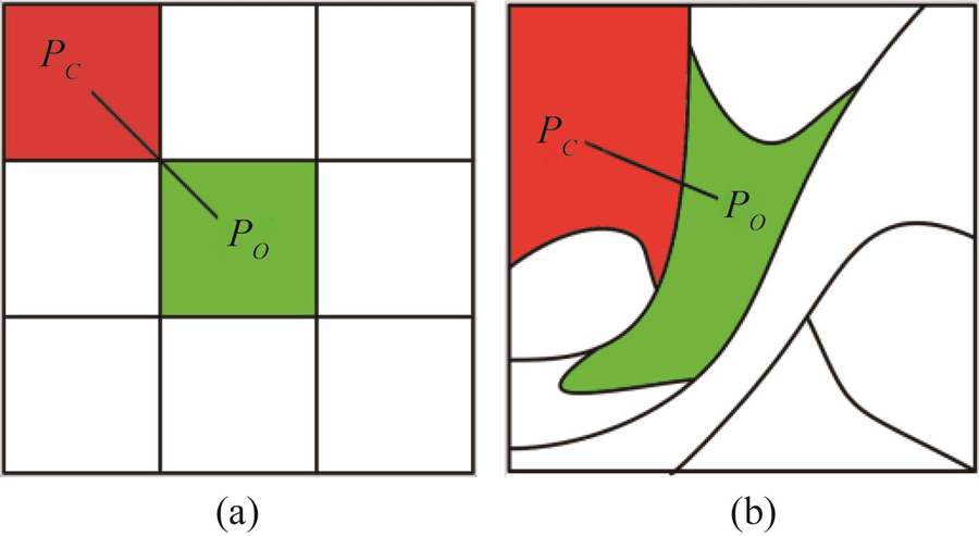
Fig. 1. Spatial information in(a)the rectangular local window and(b)the irregular scale areas

Fig. 2. The flowchart of SIISA
Fig. 3. Multispectral images covering Rome, Italy,(a)RGB of multispectral image,(b)coarse image(S=8)
Fig. 4. Hyperspectral images covering University of Pavia, Italy,(a)RGB of hyperspectral image,(b)coarse image(
Fig. 5. Hyperspectral images covering Xiong'an New Area, China,(a)RGB of hyperspectral image,(b)coarse image(
Fig. 6. Mapping results,(a)reference image,(b)SSI,(c)PSSD,(d)OSI,(e)RWA,(f)SIISA
Fig. 7. Mapping results,(a)reference image,(b)SSI,(c)PSSD,(d)OSI,(e)RWA,(f)SIISA
Fig. 8. Mapping results,(a)reference image,(b)SSI,(c)PSSD,(d)OSI,(e)RWA,(f)SIISA
Fig. 9. Salient region,(a)reference image,(b)SSI,(c)PSSD,(d)OSI,(e)RWA, and(f)SIISA
Fig. 10. Values of(a)OA(%)and(b)Kappa obtained using the five different sub-pixel methods under different values of S
Fig. 11. OA(%)value of the SIISA in relation to weight parameter
Fig. 12. OA(%)value of the SIISA in relation to segmentation scale parameter V in(a)experiments 2 and(b)3
|
Table 1. Accuracy evaluation of the five methods
|
Table 2. Accuracy evaluation of the five methods

Set citation alerts for the article
Please enter your email address
© Copyright 2018-2021 | Chinese Laser Press. All Rights Reserved 沪ICP备15018463号-20