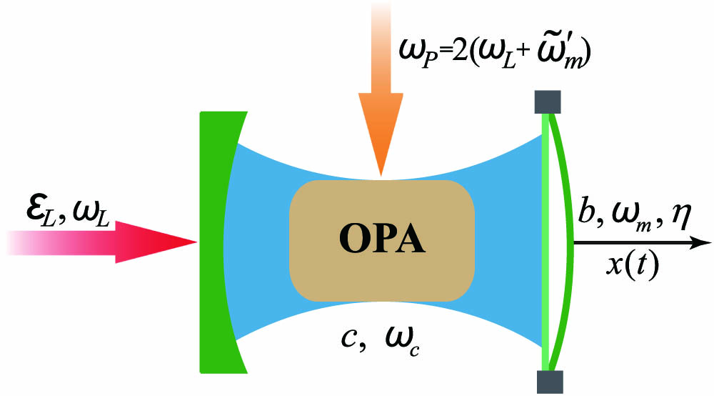
Fig. 1. Schematic diagram of the considered optomechanical system. An OPA is placed inside the cavity driven by an external laser field and is pumped by a parametric driving field. Here the movable mirror is coupled to the cavity field via the radiation-pressure interaction and is treated as a quantum-mechanical oscillator with a Duffing nonlinearity.

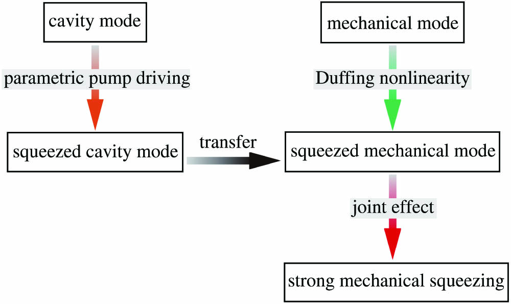
Fig. 2. Sketch of the physical processes of the joint effect between Duffing nonlinearity and parametric pump driving in construction of strong mechanical squeezing.

Fig. 3. Dependence of (a) the cavity mode phase mean square fluctuation ⟨δY2⟩ and (b) the mechanical mode position mean square fluctuation ⟨δQ2⟩ on the parametric gain G for the parametric phase θ∈[0,12π]. The horizontal dashed line represents the variance of the vacuum state. The frequency of the mechanical mode ωm/(2π)=2.5×106  Hz. Other parameters are ωc=2.5×108ωm, γm=10−6ωm, κ=0.1ωm, g0=10−4ωm, P=0.1  mW, nmth=ncth=0, and εL=2Pκ/(ℏωc).

Fig. 4. Dependence of the mechanical mode position mean square fluctuation ⟨δQ2⟩ on the parametric gain G in the cases of η=0 and η=10−5ωm. The parameter sets (G,η) corresponding to the points A, B, C, and D are (0,0), (0.4κ,0), (0,10−5ωm), and (0.4κ,10−5ωm), respectively. Here we have set θ=0, and other parameters are the same as in Fig. 3. The shadowed blue bottom region corresponds to squeezing below the 3 dB limit.

Fig. 5. Wigner function in the phase space for the mechanical mode. (a), (b), (c), and (d) correspond to the points A, B, C, and D in Fig. 4, respectively. The parameters are the same as in Fig. 4.

Fig. 6. Mechanical mode position mean square fluctuation ⟨δQ2⟩ obtained by the numerical solution in Eq. (25) and the analytical solution in Eq. (44), respectively, in the cases of η=0 and η=10−5ωm. Other parameters are the same as in Fig. 4. The shadowed blue bottom region corresponds to squeezing below the 3 dB limit.

Fig. 7. Dependence of the mechanical mode position mean square fluctuation ⟨δQ2⟩ on the thermal phonon number nmth. Here we have set κ=0.2ωm, η=10−4ωm, G=0.49κ, θ=0, and P=10  mW. Other parameters are the same as in Fig. 3. The shadowed blue bottom region corresponds to squeezing below the 3 dB limit.

Fig. 8. Contour plot of the detection spectrum SZout(ω) of the quadrature fluctuation of the output field versus the frequency ω and the measurement phase angle ϕ when G=0.4κ and η=10−5ωm. Other parameters are the same as in Fig. 4.

Table 1. Applying Either (Both) of the Parametric Pump Driving and the Duffing Nonlinearity, the Sole (Joint) Squeezing Result (in Units of Decibels) of These Two Different Squeezing Methods in Different Parameter Sets of (P,G,η)^a