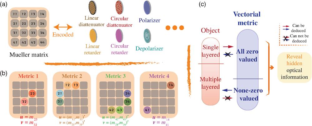
Fig. 1. MM and the asymmetric inference of vectorial metrics. (a) Different vectorial optical properties that are encoded in an MM. (b) Four vectorial metrics and related elements in their MMs. (c) A summary of the asymmetric inference network of vectorial metrics. The blue and red arrows represent the mathematical inference. Detailed explanations are in Supplementary Material 2.

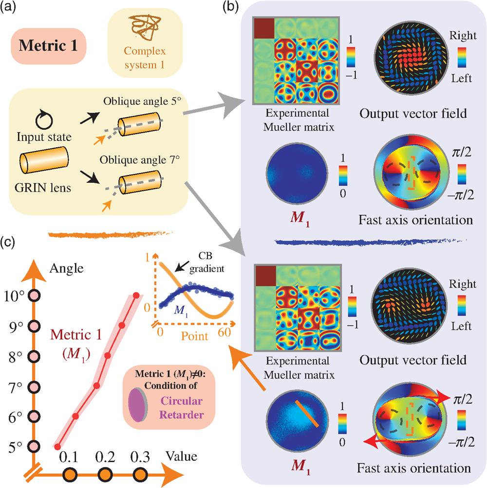
Fig. 2. GRIN lens with its decoupled vectorial information. (a) GRIN lens with right-hand circularly polarized light input, under obliquely incident angle at 5 deg and 7 deg, respectively. (b) Their related experimental MMs, output vector fields M1, fast axis orientations, as well as an example of a plot of CB gradient sampled via the yellow solid line within the subfigure of M1. (c) Value of M1 under different obliquely incident angles of this system (we use absolute value in this section for simplicity), from 5 deg to 10 deg with 1 deg interval. The value is extracted via the middle linear gradient area (orange dotted rectangle, detailed in Supplementary Material 3). The shaded area represents the standard deviation. Details of the relationship between M1 and CB can be found in Supplementary Material 2.

Fig. 3. Direct laser written waveguides with their MMs and vectorial metric analysis. (a) A sketch of the geometry of the direct laser writing process and the illumination and detection paths of the subsequent imaging process. (b) Example experimental MMs, value of metrics for waveguides written with laser pulse energies of 42 and 67 nJ, respectively. (c) The value of depolarization, M2, and polarizance of different waveguides with respect to writing pulse energy. The statistical analysis was performed on the chosen subregions (detailed in Supplementary Material 5). The shaded area represents the standard deviation. The relationship of M2 and M3 with polarization properties can be found in Supplementary Materials 2, 6, and 8.

Fig. 4. Normal/cancerous lung tissue samples with their MMs and metric information. (a) Sketches of normal lung tissue and alveoli and abnormal lung tissue with fibrosis. Demonstration for samples 1 (unstained sample and its H-E stained counterpart), showing a sketch with corresponding random sampling points in both cancerous and normal areas (see method in Supplementary Material 7). Scale bar: 50μm. (b) Experimental MMs sampled from sample C1, alongside with value of LD, LR, and M4 at two randomly chosen regions. Note the scale used for LD and LR (and related MM elements) has been amplified by a factor of 100 for better visualization. (c) Demonstration of the data from samples 1 (H1 and C1 parts); the bar chart shows the mean value and the standard deviation of M4 and retardance. Data were decomposed from the MMs for 10 points per each region of the sample. (d) A selected small region of m14 and m41 of the second cancerous MM is shown as well. This indicates the structure may have double-layered format—a sequence of linear retarder and linear diattenuator; details can be found in Supplementary Materials 1, 2, and 7.

Fig. 5. Relationships between the three spaces and passive polarization aberration compensation. (a) The complex inference network among object (space A), vectorial metrics (space B), and MM (space C). (b) Panels (i) and (ii) show a sketch of the connectivity between A, B, and C, potential new metric (M5; defined with two diagonally opposed 2×2 blocks; see details in Supplementary Material 9), as well as a demonstration of passive polarization compensation using GRIN lens and spatial half waveplate array. HWP: half wave plate. (iii) An illustration of the effect of aberration compensation. (c) Such spaces are linked with the new metric. The metric can first reveal hidden physical information of a complex system, such as uniform axis orientation in this application, then can optimize the operations, such as achieving an aberration compensated system.