
Chuan Xu, Lidan Zhang, Songtao Huang, Taxue Ma, Fang Liu, Hidehiro Yonezawa, Yong Zhang, Min Xiao. Sensing and tracking enhanced by quantum squeezing[J]. Photonics Research, 2019, 7(6): A14
- Photonics Research
- Vol. 7, Issue 6, A14 (2019)
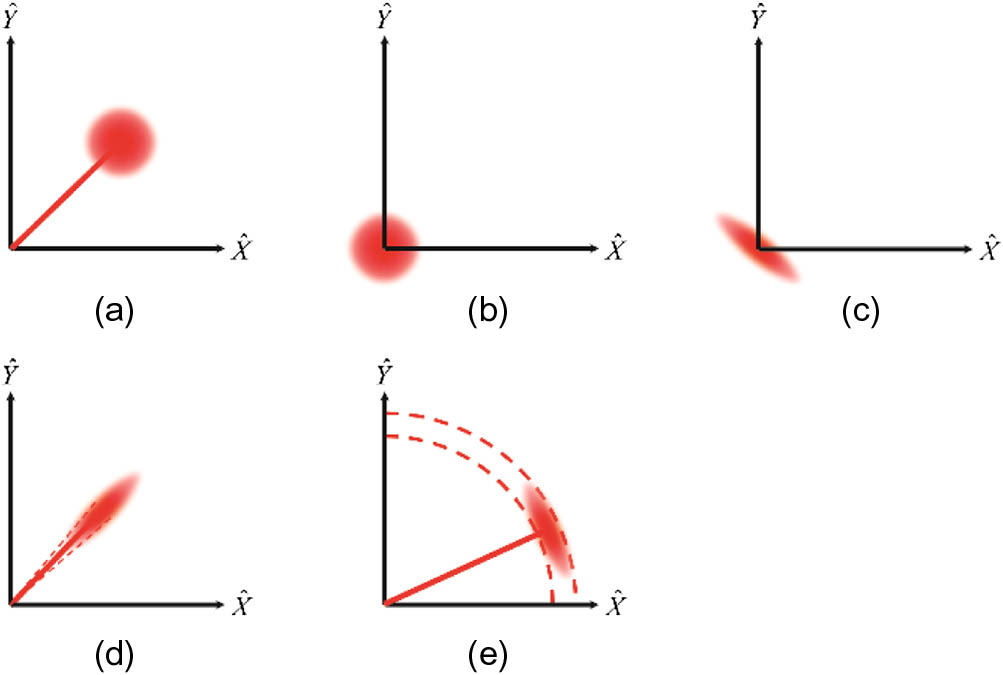
Fig. 1. Representation of different states in the phasor diagram: (a) coherent state, (b) vacuum state, (c) vacuum-squeezed state, (d) phase-squeezed state, and (e) amplitude-squeezed state.
![Schematic of degenerate OPA and graph of dielectric polarization P(E)=ε0(χ(1)E+χ(2)E2) representing the second-order nonlinear process in the crystal. Adapted with permission from Ref. [68].](/richHtml/prj/2019/7/6/06000A14/img_002.jpg)
Fig. 2. Schematic of degenerate OPA and graph of dielectric polarization P ( E ) = ε 0 ( χ ( 1 ) E + χ ( 2 ) E 2 )
Fig. 3. (a) Schematic of balanced homodyne detection. PD, photodetector. (b) Setup of an MZI. M, mirror. Coherent light illuminates port a of the MZI, while a vacuum state (or squeezed state) is injected via port b.
Fig. 4. Square-wave phase signal is obtained with (a) vacuum and (b) squeezed vacuum. Adapted with permission from Ref. [71].
Fig. 5. (a) Polarization interferometer. (b) Polarization rotation signal and noise. Adapted with permission from Ref. [72].
Fig. 6. (a) Scheme of the experiment setup in one-dimensional displacement measurement. Adapted with permission from Ref. [10]. (b) Scheme of the experiment setup in two-dimensional displacement measurement. The two squeezed modes are generated from two OPA cavities and mixed in a mode-mixing cavity. SHG, second harmonic generator; OPA, optical parametric amplifier; EOM, electro-optic modulator; ESA, electronic spectrum analyzer. Adapted with permission from Ref. [34].
Fig. 7. TEM 10
Fig. 8. (a) Schematic of squeezing-enhanced phase estimation. (b) Fisher information versus phase shift for a pure 6-dB squeezed-vacuum state. Adapted with permission from Ref. [16].
Fig. 9. (a) Dependence of estimation variance on input phase. (b) Dependence of estimation variance on the number of homodyne samples. Adapted with permission from Ref. [16].
Fig. 10. Quantum-enhanced homodyne phase tracking system. Adapted with permission from Ref. [12].
Fig. 11. (a) Dependence of MSE on squeezing level. (b) Dependence of MSE on amplitude squared | α | 2
Fig. 12. (a) Schematic of the mirror-motion estimation and (b) dependence of MSE on amplitude squared | α | 2
Fig. 13. Example of a prepared-atom ensemble where the pump beam orients the spins of the ensemble. The pump beam, probe beam, and magnetic field are mutually orthogonal. Adapted with permission from Ref. [108].
Fig. 14. Representation of quantum polarization states of bright coherent and bright amplitude-squeezed light on the Poincare sphere. Adapted with permission from Ref. [114].
Fig. 15. (a) Simplified layout of Advanced LIGO. (b) Strain noise of each detector of Advanced LIGO. Adapted with permission from Ref. [118].
Fig. 16. Simplified setup of the H1 interferometer with vacuum-squeezed-state injection. Adapted with permission from Ref. [14].
Fig. 17. Strain sensitivity of H1 detector with and without squeezed-vacuum injection. Adapted with permission from Ref. [14].
Fig. 18. Sagnac interferometer output signal. Adapted with permission from Ref. [36].
Fig. 19. (a) Dependence of phase noise reduction on frequency for the quantum-enhanced fiber interferometer. (b)–(d) Demodulated noise spectra of the interferometer output at 30 kHz, 80 kHz, and 150 kHz. Adapted with permission from Ref. [37].
Fig. 20. Time domain results of fiber-optic phase tracking. Adapted with permission from Ref. [135].

Set citation alerts for the article
Please enter your email address
© Copyright 2018-2021 | Chinese Laser Press. All Rights Reserved 沪ICP备15018463号-20