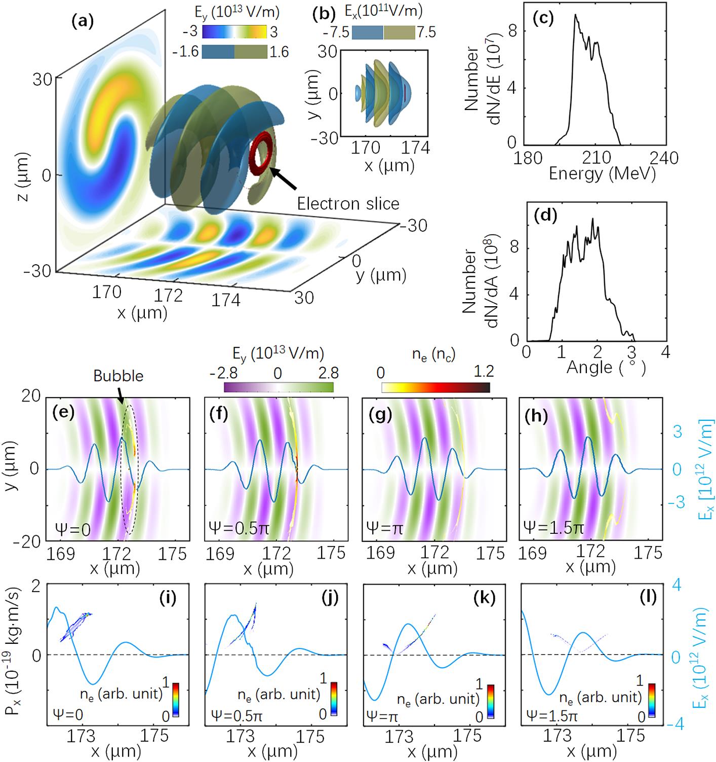
Fig. 1. Electron slice and LG laser field in PIC simulation. (a) Sketch of an electron slice driven by an LG laser. The red donut indicates the isosurface of the electron slice with n_e = 0.3n_c for the carrier-envelope Ψ = 0. The blue and yellow translucence isosurfaces indicate the distributions of the LG laser field E_y. (b) Distributions of the laser electric field E_x and electron slice in the x–y plane. (c), (d) Energetic spectra and angular distribution for the electrons in the regions of 173 μm < x < 183 μm, 0 < r < 8 μm at t = 88T. Density distributions of the electron slice for different CEPs (e) Ψ = 0, (f) 0.5π, (g) π and (h) 1.5π at 88T. Corresponding phase-space distributions of the electrons and amplitude of E_x (blue line) on the x-axis at t = 88T are plotted for (i) Ψ = 0, (j) 0.5π, (k) π and (l) 1.5π.

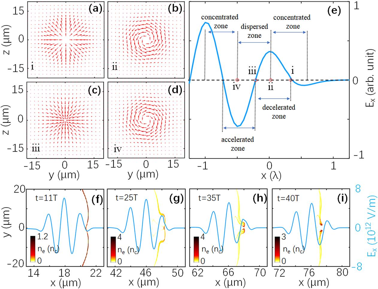
Fig. 2. Structure of electric fields of CP LG laser and phase-space distribution of electrons. Normalized vector plots of the transverse electric fields in one laser cycle for (a) point i, (b) point ii, (c) point iii, and (d) point iv marked in (e). (e) Normalized amplitude of E_x (blue line) on the x-axis for Ψ = 0. Density distributions of electron slice and amplitude of E_x (blue solid) for Ψ = 0 at (f) t = 11T, (g) t = 25T, (h) t = 35T, and (i) t = 40T are plotted.

Fig. 3. Trajectories of electrons in a single-particle model and AM in PIC simulation. (a) 3D trajectories of electrons at different initial positions of x = 3.8 μm [accelerated phase corresponding to point iv in Figure 2(e)], y = ±1 μm, and z = ±1 μm. Here, the electrons have an initial velocity of v_x = 0.999c. (b) AM for the electrons in the regions of 0 μm < x < 400 μm, −10 μm < y < 10 μm, and −10 μm < z < 10 μm in PIC simulation with Ψ = 0. (c) View of 3D trajectories in the forward direction.

Fig. 4. Comparisons between the cases driven by LG laser and Gaussian laser. Density distributions of electrons at t = 853 fs for (a) LG laser with λ = 2 μm, (b) LG laser with λ = 0.8 μm, and (c) Gaussian laser with λ = 2 μm. (d)–(f) Energetic spectra and (g)–(i) angular distribution of the electrons in (a)–(c), respectively. The electrons in in the regions of 252.8 μm < x < 260 μm, 0 < r < 10 μm are considered for the cases in (d) and (g) and the electrons in the regions of 250 μm < x < 260 μm, 0 < r < 20 μm are considered for the cases in (e), (f), (h), and (i).