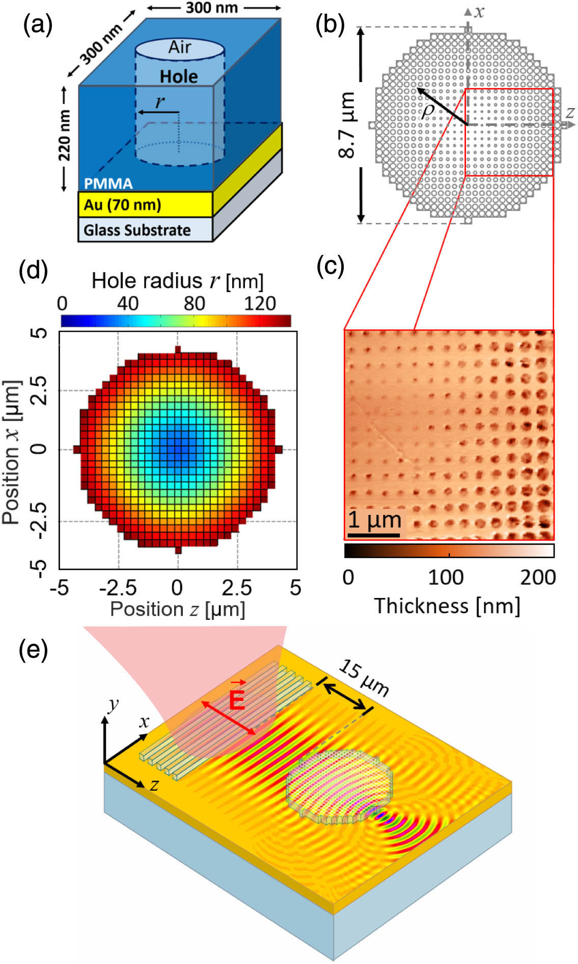
Fig. 1. Schematic diagrams of (a) the elementary unit cell that conforms the PMLL and (b) the whole PMLL structure. (c) High-resolution atomic-force microscopy image of a 4 μm×4 μm area taken on top of the PMLL. (d) Radii size distribution of every elementary unit cell. (e) Schematic diagram (not at scale) showing the PMLL and the grating used to excite the SPPs, which propagate in the z direction. The red double arrow indicates the polarization of the laser.

Fig. 2. (a) Designed and analytical values of the local effective-mode index as a function of the relative position z, where z=0 corresponds to the center of the PMLL, and δ=1.3  μm corresponds to the difference between the limit of the physical lens (blue) and the Luneburg radius R_L (red). (b) and (c) Calculated values of the (b) real and (c) imaginary parts of the designed local effective-mode index. (d) Dependence of the effective mode index nm of SPPs in the multilayer system for different values of the PMMA thickness. (e) Optical losses in the PMLL at each point of the structure.

Fig. 3. The calculated (a) field and (b) intensity distributions of SPPs propagating along z and passing through an ideal 2D Luneburg lens (continuum case). The red circles indicate the radius RL of the Luneburg lens. (c) Transverse cross section of the intensity profile at the point ρ=RL. The calculated (d) field and (e) intensity distributions of SPPs propagating through the designed PMLL (discrete case). The physical limits of the lens are delimited with black contours. (f) Transverse cross section showing the FWHM at the point ρ=RL.

Fig. 4. (a) LRM image of the SPP intensity distribution as it passes through the PMLL with symmetrical illumination conditions with respect to the radial axis. The inset corresponds to the intensity profile cross section at the focal point. (b) and (c) LRM images of the SPP intensity distributions with asymmetrical illumination. The dashed white circles correspond to the PMLL theoretical radius RL=10  μm. The asymmetric illumination is produced by displacing the beam a distance (b) d1=2.5  μm and (c) d2=2.0  μm from the radial axis.

Fig. 5. (a) LRM cropped image of the Fourier plane. The origin (κx,κz)=(0,0) is located in the center of the bright spot to the left of the image. (b) Intensity cross section along κz for κx=0. Each peak corresponds to different values of the effective mode indices supported in the PMLL.

Fig. 6. (a) LRM interference pattern of the SPPs that propagate and interact with the PMLL and interfere with a reference beam. (b) Measured phase distribution obtained from the interference pattern in (a). (c) Calculated amplitude of a plane wave interacting with the designed PMLL simulated with the BPM.

Fig. 7. (a) LRM setup with an illumination scheme that focuses the excitation beam onto the grating to generate SPPs. (b) Modified experimental setup, which illuminates the whole area of interest to generate interference patterns in the image plane. The incident light acts as a reference beam and interferes with the leakage radiation (LR) of the excited SPPs generated with the grating. The schematic diagram shows how the LR recombines with the reference beam to generate the interference pattern in the image plane.

Fig. 8. (a) Pixel intensity values for a row of pixels along the propagation direction. (b) Average-subtracted intensity values. The dashed lines correspond to the numerical fit to the maximum and minimum values. (c) Normalized signal and corresponding SPP phase.

Table 1. Measured Effective Refractive Indices